Flexible Fitting Tutorial, Part II
|
The tutorial introduces the
basic
ideas of the older (Situs 2.x era) feature point or skeleton--based flexible
docking strategies using actin and RNA Polymerase test systems.
It
is helpful for the
understanding
of the tutorial if the user is already familiar with the classic
EM tutorial and the correlation-based docking tutorial. To simplify the modeling we use the qplasty
tool for approximative flexing at a carbon alpha level of detail. We
offer alternative (and more stereochemically accurate) Molecular
Dynamics protocols at Situs Flavors. The
results of the flexing can
be compared to solutions
distributed with the tutorial software. More documentation is available
in the user
guide, on the methodology
page, and in the published
articles.
It is helpful
for the
understanding
of the tutorial if the user has performed
at least the installation
step of part I (the rest of part I can be skipped if the
earlier
output files are copied from the "solutions" directory). |
Content:
|
Data
Flow and Design
The
series
of steps and the programs that are required to dock an
atomic-resolution
structure flexibly to single-molecule, low-resolution data are shown
schematically
in the following figure. Detailed program explanations
are
given
in the user guide .
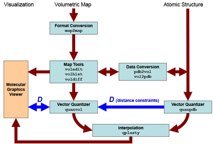
Schematic
diagram of flexing related
routines. Major Situs components (blue) are classified by their
functionality.
The main work flow is indicated by brown arrows. The advanced modeling
of
distance constraints for the motion
capture skeleton is
shown in dark
blue. Visualization
(orange) for the rendering of the data requires a molecular
graphics viewer (we
use
here the
VMD
graphics program,
Chimera and Sculptor also
support Situs
format).
Standard EM
formats are supported
and are converted to cubic lattices in Situs format. This is done with
the map2map
utility. Subsequently, the
data is inspected and, if necessary, prepared for the vector
quantization using a variety of visualization and analysis
tools.
Atomic
coordinates in PDB format can be transformed to low-resolution maps, if
necessary, and vice versa. During vector quantization of the
high-resolution structure,
distances can be learnt that are sent to the vector quantizer of the
low-resolution
structure to enable skeleton-based
fitting.
After
the vector quantization, the high-resolution structure is flexibly
docked by the qplasty
tool to
the
low-resolution density by the
corresponding codebook
vectors.
|
| Creating
a Simulated Target Map for Validation
First
we create
a simulated EM map from a known atomic structure for later validation.
We lower the
resolution of the
target structure to 15 Å with the pdb2vol
kernel convolution utility. Enter at the shell prompt:
| ./pdb2vol
0_actin_target.pdb
1_actin_target.situs |
Select
mass-weighting (enter 2)
and select no B-factor cutoff (enter 1). Next enter the desired voxel
spacing of the output map. Given the dimensions of the structure, 2
Å
appears to be a good compromise between lattice accuracy and storage
requirement.
Next, enter the desired output resolution as a negative number: -15
Å.
Next, select the Gaussian smoothing kernel (enter 1). Select lattice
correction
(enter 1), and enter the maximum amplitude of the kernel (enter
1). You can also automate this
procedure in a script by overloading the expected input (see run_tutorial.bash for
details):
The program
projects the atomic
structure to the lattice, computes the Gaussian kernel, and carries out
the real-space convolution, writing the resulting volumetric map to the
file 1_actin_target.situs.
Here is the full program
output:
./pdb2vol
0_actin_target.pdb 1_actin_target.situs
lib_pio>
3572 atoms read.
pdb2vol>
Found 639 hydrogens, 0 water atoms, 0 codebook vectors, 0 density atoms
pdb2vol>
Hydrogens will be ignored.
pdb2vol>
Do you want to mass-weight the atoms ?
pdb2vol>
pdb2vol>
1: No
pdb2vol>
2: Yes
pdb2vol>
2
pdb2vol>
Do you want to select atoms based on a B-factor threshold?
pdb2vol>
pdb2vol>
1: No
pdb2vol>
2: Yes
pdb2vol>
1
pdb2vol>
2933 out of 3572 atoms selected for conversion.
pdb2vol>
pdb2vol>
The input structure measures 74.971 x 62.460 x 38.249 Angstrom
pdb2vol>
pdb2vol>
Please enter the desired voxel spacing for the output map (in
Angstrom): 2
pdb2vol>
pdb2vol>
Kernel width. Please enter (in Angstrom):
pdb2vol>
(as pos. value) kernel half-max radius or
pdb2vol>
(as neg. value) target resolution (2 sigma)
pdb2vol>
Now enter (signed) value: -15
pdb2vol>
pdb2vol>
Please select the type of smoothing kernel:
pdb2vol>
pdb2vol>
1: Gaussian, exp(-1.5 r^2 / sigma^2)
pdb2vol>
sigma = 7.500A, r-half = 5.098A, r-cut = 12.990A
pdb2vol>
pdb2vol>
2: Triangular, max(0, 1 - 0.5 |r| / r-half)
pdb2vol>
sigma = 7.500A, r-half = 5.929A, r-cut = 11.859A
pdb2vol>
pdb2vol>
3: Semi-Epanechnikov, max(0, 1 - 0.5 |r|^1.5 / r-half^1.5)
pdb2vol>
sigma = 7.500A, r-half = 7.331A, r-cut = 11.637A
pdb2vol>
pdb2vol>
4: Epanechnikov, max(0, 1 - 0.5 r^2 / r-half^2)
pdb2vol>
sigma = 7.500A, r-half = 8.101A, r-cut = 11.456A
pdb2vol>
pdb2vol>
5: Hard Sphere, max(0, 1 - 0.5 r^60 / r-half^60)
pdb2vol>
sigma = 7.500A, r-half = 9.722A, r-cut = 9.835A
pdb2vol>
1
pdb2vol>
pdb2vol>
Do you want to correct for lattice interpolation smoothing effects?
pdb2vol>
pdb2vol>
1: Yes (slightly lowers the kernel width to maintain target resolution)
pdb2vol>
2: No
pdb2vol>
1
pdb2vol>
pdb2vol>
Finally, please enter the desired kernel amplitude (scaling factor): 1
pdb2vol>
pdb2vol>
Projecting atoms to cubic lattice by trilinear interpolation...
pdb2vol>
... done. Lattice smoothing (sigma = atom rmsd): 1.408 Angstrom
pdb2vol>
pdb2vol>
Computing Gaussian kernel (correcting sigma for lattice smoothing)...
pdb2vol>
... done. Kernel map extent 15 x 15 x 15 voxels
pdb2vol>
pdb2vol>
Convolving lattice with kernel...
pdb2vol>
... done. Spatial resolution (2 sigma) of output map: 15.000A
pdb2vol>
lib_vio>
Writing density data...
lib_vio>
Volumetric data written to file 1_actin_target.situs
lib_vio>
Situs formatted map file 1_actin_target.situs - Header information:
lib_vio>
Columns, rows, and sections: x=1-57, y=1-52, z=1-39
lib_vio>
3D coordinates of first voxel (1,1,1):
(-58.000000,-50.000000,-36.000000)
lib_vio>
Voxel size in Angstrom: 2.000000
|
By loading the resulting map
into VMD
(see below), one can vary the density threshold. A threshold of
10 (~15% of the maximum value) corresponds approximately to the surface
of the molecule.
|
| Preliminary
Rigid-Body Registration
Before we start
fitting the original
actin structure to the target structure, it is important to roughly
align
the atomic structure and the target map by rigid-body fitting.
An initial alignment
"by eye" can e.g. be done with VMD (move a
loaded molecule by selecting the VMD menu Mouse -> Move
->
Molecule,
then translate it with the mouse and rotate it by pressing the Shift
key; the new coordinates can then be saved by selecting File ->
Save
Coordinates).
Alternatively, an automated
rigid-body fitting
procedure can also be employed, e.g. using colores, collage, or matchpt as explained in
other tutorials.
It is a good idea to
export a
number
of best-scoring rigid body fits, and
to explore the alignment of these
fits by eye, before selecting one for subsequent flexible fitting.
For
example,
using colores at the shell prompt enter:
| ./colores
1_actin_target.situs
0_actin_orig.pdb -res
15.0
-deg 20 -explor 1 |
After this run
we rename the resulting fit and remove the auxiliary files of the
colores run:
mv
col_best_001.pdb 2_actin_orig_dock_target.pdb
rm col_*
|
|
| Vector
Quantization of the High-Resolution Structure with quanpdb
Now, we perform
the vector quantization
of the rigid fitted structure with the quanpdb
utility.
At the shell
prompt, enter
| ./quanpdb
2_actin_orig_dock_target.pdb
2_actin_orig_dock_target.qpdb |
and select mass-weighting
(enter 2),
ignore the B-factor cutoff (enter 1). Next, enter the
number
of codebook vectors: 4 (one for each of actin's subdomains). Watch the
program compute a number of datasets for statistical
averaging.
The file 2_actin_orig_dock_target.qpdb now contains the four new
codebook
vectors, their rms variability, and the effective radius of their Voronoi
cells, in PDB format. Finally, the user is asked whether
nearest-neighbor
connectivities should be learnt, or whether the Voronoi cells should be
saved. Here we twice enter 1 (don't save the connectivities or Voronoi
cells). See also run_tutorial.bash.
Here is the
output of the entire
quanpdb calculation:
./quanpdb
2_actin_orig_dock_target.pdb 2_actin_orig_dock_target.qpdb
lib_pio>
3580 atoms read.
quanpdb>
Found 639 hydrogens, 0 water atoms, 8 codebook vectors, 0 density atoms
quanpdb>
Hydrogens will be ignored.
quanpdb>
Do you want to mass-weight the atoms ?
quanpdb>
quanpdb>
1: No
quanpdb>
2: Yes
quanpdb>
2
quanpdb>
Do you want to select atoms based on a B-factor threshold?
quanpdb>
quanpdb>
1: No
quanpdb>
2: Yes
quanpdb>
1
quanpdb>
2954 equally weighted inputs out of originally 3580 atoms selected for
conversion.
quanpdb>
quanpdb>
Sphericity of the atomic structure: 0.52
quanpdb>
Enter desired number of codebook vectors for data quantization: (0 to
exit): 4
quanpdb>
Computing 8 datasets, 100000 iterations each...
quanpdb>
Now producing dataset 1
quanpdb>
Now producing dataset 2
quanpdb>
Now producing dataset 3
quanpdb>
Now producing dataset 4
quanpdb>
Now producing dataset 5
quanpdb>
Now producing dataset 6
quanpdb>
Now producing dataset 7
quanpdb>
Now producing dataset 8
quanpdb>
quanpdb>
Codebook vectors have been written to file
2_actin_orig_dock_target.quanpdb
quanpdb>
The PDB B-factor field contains the equivalent spherical radii
quanpdb>
of the corresponding Voronoi cells (in Angstrom).
quanpdb>
Cluster analysis of the 8 independent calculations:
quanpdb>
The PDB occupancy field in 2_actin_orig_dock_target.qpdb contains the
rms variabilities of the vectors.
quanpdb>
Average rms fluctuation of the 4 codebook vectors: 0.865 Angstrom
quanpdb>
Radius of gyration of the 4 codebook vectors: 17.347 Angstrom
quanpdb>
quanpdb>
Do you want to learn nearest-neighbor connectivities?
quanpdb>
Choose one of the following options -
quanpdb>
1: No.
quanpdb>
2: Learn and save to a PSF file
quanpdb>
3: Learn and save to a constraints file
quanpdb>
4: Learn and save to both PSF and constraints files
quanpdb>
1
quanpdb>
quanpdb>
Do you want to save the Voronoi cells?
quanpdb>
Choose one of the following options -
quanpdb>
1: No.
I'm done
quanpdb>
2: Yes. Save cells to a PDB file
quanpdb>
1
quanpdb> Bye bye!
|
|
| Vector
Quantization of the Low-Resolution Map with quanvol
For the vector
quantization of the volumetric
dataset with the quanvol
utility we use
the previous quanpdb codebook vectors as start positions. After entering
./quanvol
1_actin_target.situs 2_actin_orig_dock_target.qpdb
\
3_actin_target.qvol |
the user is
prompted to enter
the density cutoff value. We enter 100 which is an appropriate surface
value for this map. Subsequently, the program
asks whether we wish to optimize the data. or analyse it only. We enter
1 for LBG optimization. Next, the program asks if the users wishes to
use distance constraints, we enter 1 (No). Finally, the user is asked
whether
nearest-neighbor connectivities should be learnt. For now we enter 1
(No). The file
3_actin_target.qvol
now contains the codebook vectors.
Here is the
output of this quanvol
calculation:
./quanvol
1_actin_target.situs 2_actin_orig_dock_target.qpdb 3_actin_target.qvol
lib_vio> Situs formatted map file 1_actin_target.situs
- Header information:
lib_vio> Columns, rows, and sections: x=1-57, y=1-52, z=1-39
lib_vio> 3D coordinates of first voxel:
(-58.000000,-50.000000,-36.000000)
lib_vio> Voxel size in Angstrom: 2.000000
lib_vio> Reading density data...
lib_vio> Volumetric data read from file 1_actin_target.situs
quanvol> Density values below a user-defined cutoff value will
not be considered
quanvol> Do you want to inspect the input density values before
entering the cutoff value?
quanvol> Choose one of the following three options -
quanvol> 1: No
(continue)
quanvol> 2:
Show me the minimum and maximum density values only
quanvol> 3:
Show me the voxel histogram
quanvol> 1
quanvol> Now enter the cutoff density value: 100
quanvol> Cutting off density values < 100.000000,
remaining occupied volume: 12713 voxels (1.017040e+05 Angstrom^3)
lib_pio> 4 atoms read.
quanvol> Do you want to optimize the start vectors or skip and
proceed to the connectivity analysis?
quanvol> Choose one of the following two options -
quanvol> 1:
Optimize start vectors with LBG
quanvol> 2:
Skip and proceed directly to connectivity analysis
quanvol> 1
quanvol>
quanvol> Using start vectors from file
2_actin_orig_dock_target.qpdb.
quanvol>
quanvol> Vector distance constraints restrict undesired degrees
of freedom.
quanvol> Do you want to add distance constraints?
quanvol> Choose one of the following three options -
quanvol> 1: No
quanvol> 2:
Yes. I want to enter them manually
quanvol> 3:
Yes. I want to read connectivities from a PSF file and use start vector
distances
quanvol> 4:
Yes. I want to read them from a Situs constraints file
quanvol> 1
quanvol> Starting standard LBG vector quantization.
quanvol> It. 1 -- Average vector update: 3.794887e-01 Angstrom
quanvol> It. 2 -- Average vector update: 3.459883e-01 Angstrom
quanvol> It. 3 -- Average vector update: 3.164652e-01 Angstrom
quanvol> It. 4 -- Average vector update: 2.914341e-01 Angstrom
quanvol> It. 5 -- Average vector update: 2.667951e-01 Angstrom
quanvol> It. 6 -- Average vector update: 2.440749e-01 Angstrom
quanvol> It. 7 -- Average vector update: 2.238978e-01 Angstrom
quanvol> It. 8 -- Average vector update: 2.044688e-01 Angstrom
quanvol> It. 9 -- Average vector update: 1.876906e-01 Angstrom
quanvol> It. 10 -- Average vector update: 1.723334e-01 Angstrom
quanvol> It. 11 -- Average vector update: 1.587836e-01 Angstrom
quanvol> It. 12 -- Average vector update: 1.464327e-01 Angstrom
quanvol> It. 13 -- Average vector update: 1.345356e-01 Angstrom
quanvol> It. 14 -- Average vector update: 1.241281e-01 Angstrom
quanvol> It. 15 -- Average vector update: 1.145233e-01 Angstrom
quanvol> It. 16 -- Average vector update: 1.052219e-01 Angstrom
quanvol> It. 17 -- Average vector update: 9.707859e-02 Angstrom
quanvol> It. 18 -- Average vector update: 8.882026e-02 Angstrom
quanvol> It. 19 -- Average vector update: 8.154858e-02 Angstrom
quanvol> It. 20 -- Average vector update: 7.512557e-02 Angstrom
quanvol> It. 21 -- Average vector update: 6.959220e-02 Angstrom
quanvol> It. 22 -- Average vector update: 6.432284e-02 Angstrom
quanvol> It. 23 -- Average vector update: 5.972955e-02 Angstrom
quanvol> It. 24 -- Average vector update: 5.495829e-02 Angstrom
quanvol> It. 25 -- Average vector update: 5.124211e-02 Angstrom
quanvol> It. 26 -- Average vector update: 4.685754e-02 Angstrom
quanvol> It. 27 -- Average vector update: 4.316624e-02 Angstrom
quanvol> It. 28 -- Average vector update: 4.039170e-02 Angstrom
quanvol> It. 29 -- Average vector update: 3.792771e-02 Angstrom
quanvol> It. 30 -- Average vector update: 3.597380e-02 Angstrom
quanvol> It. 31 -- Average vector update: 3.496715e-02 Angstrom
quanvol> It. 32 -- Average vector update: 3.241709e-02 Angstrom
quanvol> It. 33 -- Average vector update: 3.048423e-02 Angstrom
quanvol> It. 34 -- Average vector update: 2.848838e-02 Angstrom
quanvol> It. 35 -- Average vector update: 2.647463e-02 Angstrom
quanvol> It. 36 -- Average vector update: 2.404363e-02 Angstrom
quanvol> It. 37 -- Average vector update: 2.244006e-02 Angstrom
quanvol> It. 38 -- Average vector update: 2.056871e-02 Angstrom
quanvol> It. 39 -- Average vector update: 1.959148e-02 Angstrom
quanvol> It. 40 -- Average vector update: 1.851113e-02 Angstrom
quanvol> It. 41 -- Average vector update: 1.725249e-02 Angstrom
quanvol> It. 42 -- Average vector update: 1.626679e-02 Angstrom
quanvol> It. 43 -- Average vector update: 1.602147e-02 Angstrom
quanvol> It. 44 -- Average vector update: 1.627645e-02 Angstrom
quanvol> It. 45 -- Average vector update: 1.567052e-02 Angstrom
quanvol> It. 46 -- Average vector update: 1.466849e-02 Angstrom
quanvol> It. 47 -- Average vector update: 1.390725e-02 Angstrom
quanvol> It. 48 -- Average vector update: 1.287678e-02 Angstrom
quanvol> It. 49 -- Average vector update: 1.187649e-02 Angstrom
quanvol> It. 50 -- Average vector update: 1.093469e-02 Angstrom
quanvol> It. 51 -- Average vector update: 1.013612e-02 Angstrom
quanvol> It. 52 -- Average vector update: 9.438498e-03 Angstrom
quanvol>
quanvol> Final clustering -- Average vector update: 0.000000e+00
Angstrom
quanvol>
quanvol> Codebook vectors have been written to file
3_actin_target.qvol
quanvol> The PDB B-factor field contains the equivalent
spherical radii
quanvol> of the corresponding Voronoi cells (in Angstrom).
quanvol> Radius of gyration of the 4 codebook vectors: 19.685
Angstrom
quanvol>
quanvol> Do you want to update or save the input connectivities?
quanvol> Choose one of the following options -
quanvol> 1:
No. I'm done
quanvol> 2:
Update and save to a PSF file
quanvol> 3:
Update and save to a constraints file
quanvol> 4:
Update and save to both PSF and constraints files
quanvol> 1
quanvol> Bye bye!
|
|
| Flexible
Fitting using
Interpolation
The flexible
docking is approximated, based on the sparsely sampled displacements
from the above quanvol and quanpdb codebook vectors, by interpolation
with qplasty. This is sufficient for
carbon alpha
level accuracy. We use here the default parameters for qplasty. For more information on the
algorithm
see Rusu
et al., 2008.
To start the flexing,
enter at the shell prompt:
./qplasty
2_actin_orig_dock_target.pdb
2_actin_orig_dock_target.qpdb \
3_actin_target.qvol 4_flexed_to_target.pdb
|
The flexed structure has
been written
to file 4_flexed_to_target.pdb.
|
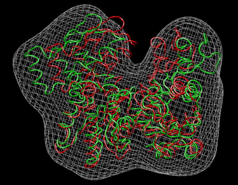
Visualization (Actin)
We inspect the above
results with VMD. The following
sequence of commands
in the VMD text console (cf. VMD
user guide) will load the original and flexed actin
structures,
2_actin_orig_dock_target.pdb (red) and 4_flexed_to_target.pdb (green),
and render them in colored tube representation. The script also renders
the target
density
map, 1_actin_target.situs, in gray:
mol load
pdb 4_flexed_to_target.pdb
mol load
pdb 2_actin_orig_dock_target.pdb
mol load
situs 1_actin_target.situs
mol top 0
rotate
stop
display
resetview
display
projection orthographic
mol
modstyle
0 0 Tube 0.3 6
mol
modstyle
0 1 Tube 0.3 6
mol
modstyle
0 2 Isosurface 100 0 0 1 2 1
mol
modcolor 0 0 ColorID 7
mol
modcolor 0 1 ColorID 1
mol
modcolor 0 2 ColorID 2
|
Don't forget to hit "enter"
after the last line! The result
should look very similar to this image:
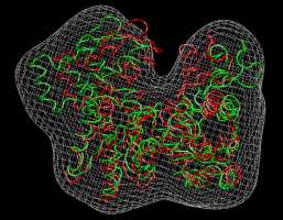
(Click
image to
enlarge)
|
| Introduction to Skeletons
The above example using four feature points is very elementary. To
improve the
stereochemical quality of the flexing, it is possible to constrain the
distances between the features to reduce the effect of noise and
experimental
limitations on the codebook vector positions. This "skeleton" based
approach, as
described on the Vector
Quantization
page, is related to 3D
motion capture
technology
used in the entertainment industry and in biomechanics.
In principle, the resolution
of
flexible fitting of an atomic structure to a low-resolution map could be
improved by increasing the number of codebook
vectors. However, one cannot increase the level of detail indefinitely. If there
are
experimental limitations
(e.g. noise, missing parts) not all vectors converge towards equivalent
features in the two data sets at a higher level of detail.
The solution to this problem is to freeze
longitudinal
degrees of freedom, and to impose distance constraints on the
vectors.
We consider here an
interesting case,
the
flexible fitting of the closed RNA polymerase structure to a
(simulated) open form at low resolution. Inspection of this file
reveals that an isocontour value of 50 units is appropriate. Important: Before
we start the
flexing, it is again mandatory to roughly
align the atomic structure and the target map by rigid-body fitting.
This
can be done "by eye" or with one of our Situs tools, as described above. Here the structures are
already
sufficiently aligned, but it isn't always the case.
|
| Vector
Quantization of the High-Resolution Structure
Now, we perform the vector
quantization of the roughly aligned atomic structure with the quanpdb
utility.
At the shell prompt, enter
| ./quanpdb
0_rnap1.pdb 5_rnap1.qpdb |
and select mass weigthing (enter 2) and no B-factor cutoff (enter 1).
Next, enter the number
of codebook vectors: 15. Watch the program compute a number of datasets
for statistical averaging. The file 5_rnap1.qpdb
now contains the 15 new codebook vectors, their rms variability, and
the effective radius of their Voronoi
cells, in
PDB format. Finally, the user is asked whether nearest-neighbor
connectivities
should be learnt, or whether the Voronoi cells should be saved. Here we
enter 2 to save the connectivities to file 5_rnap1.qpsf.
We do not wish to save the Voronoi cells (enter 1).
Here
is the
output of the entire
quanpdb calculation:
./quanpdb
0_rnap1.pdb 5_rnap1.qpdb
lib_pio>
10760
atoms read.
quanpdb>
Found
0 hydrogens, 0 water atoms, 0 codebook vectors, 0
density atoms
quanpdb>
Do you
want to mass-weight the atoms ?
quanpdb>
quanpdb>
1: No
quanpdb>
2: Yes
quanpdb>
2
quanpdb>
Do you
want to select atoms based on a B-factor threshold?
quanpdb>
quanpdb>
1: No
quanpdb>
2: Yes
quanpdb>
1
quanpdb>
10760
equally weighted inputs out of originally 10760 atoms
selected for conversion.
quanpdb>
quanpdb>
Sphericity of the atomic structure: 0.20
quanpdb>
Enter
desired number of codebook vectors for data
quantization: (0 to exit): 15
quanpdb>
Computing 8 datasets, 100000 iterations each...
quanpdb>
Now
producing dataset 1
quanpdb>
Now
producing dataset 2
quanpdb>
Now
producing dataset 3
quanpdb>
Now
producing dataset 4
quanpdb>
Now
producing dataset 5
quanpdb>
Now
producing dataset 6
quanpdb>
Now
producing dataset 7
quanpdb>
Now
producing dataset 8
quanpdb>
quanpdb>
Codebook vectors have been written to file 5_rnap1.qpdb
quanpdb>
The
PDB B-factor field contains the equivalent spherical
radii
quanpdb>
of the
corresponding Voronoi cells (in Angstrom).
quanpdb>
Cluster analysis of the 8 independent calculations:
quanpdb>
The
PDB occupancy field in 5_rnap1.quanpdb contains the rms
variabilities of the vectors.
quanpdb>
Average rms fluctuation of the 15 codebook vectors: 3.732 Angstrom
quanpdb>
Radius
of gyration of the 15 codebook vectors: 41.810
Angstrom
quanpdb>
quanpdb>
Do you
want to learn nearest-neighbor connectivities?
quanpdb>
Choose
one of the following options -
quanpdb>
1: No.
quanpdb>
2:
Learn and save to a PSF
file
quanpdb>
3:
Learn and save to a
constraints file
quanpdb>
4:
Learn and save to both PSF
and constraints files
quanpdb>
2
quanpdb>
Enter
PSF filename: 5_rnap1.qpsf
quanpdb>
Connectivity data written to PSF file 5_rnap1.qpsf.
quanpdb>
quanpdb>
Do you
want to save the Voronoi cells?
quanpdb>
Choose
one of the following options -
quanpdb>
1: No.
I'm done
quanpdb>
2:
Yes. Save cells to a PDB
file
quanpdb>
1
quanpdb>
Bye
bye..
|
|
| Assigning
Corresponding Vectors and Distance Constraints
We now have codebook vectors
and the
distance information for the atomic structure. To proceed with the
flexible docking, two problems
must be solved:
- We
need to
generate low-resolution vectors that are in correspondance with
the atomic ones, i.e. here we must form 15 pairs
of vectors that will be used as refinement parameters.
- Modeling
of
the
skeleton. The distance
connectivity file 5_rnap1.qpsf contains connectivity information about
adjacent high-resolution vectors. This file is only a starting point.
E.g. enforcing all of these constraints
would
make the structure rather rigid, so we must select a sparse set of
non-redundant
distances, i.e. a skeleton, that enables flexible fitting.
There
is no
automated
Situs routine for assigning corresponding vectors and for modeling the
skeleton. It is recommended to select these vectors by visual
inspection
with a graphics program.
Vector
connectivities in PSF format
(recognized by Molecular Dynamics related programs such as VMD, CHARMM,
X-PLOR, CNS, NAMD) can be visualized and edited as bond connections
(together with the
corresponding codebook vector PDB file) using the molecular graphics
program VMD.
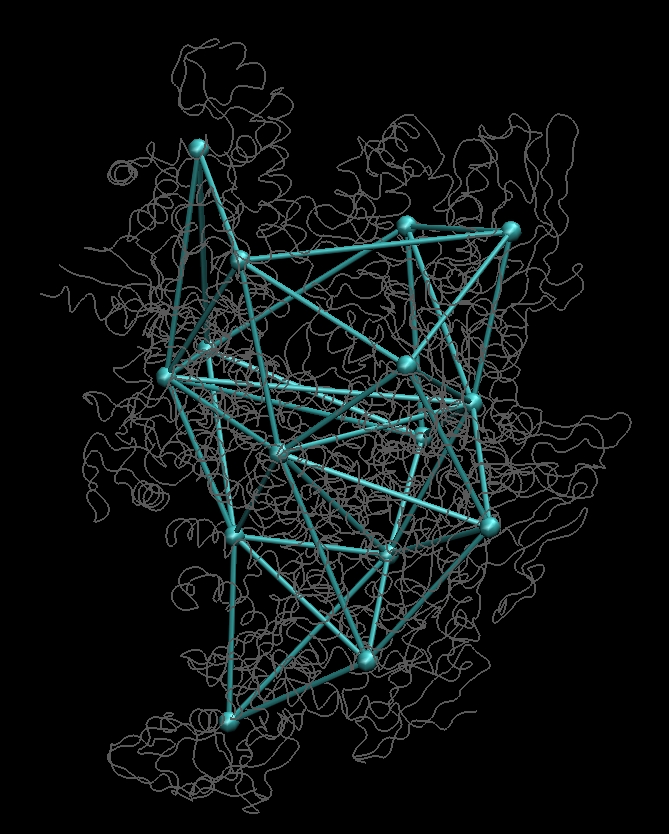
Here we
overload
the
PSF file into the PDB file in the VMD command console:
mol load
pdb
5_rnap1.qpdb psf 5_rnap1.qpsf
mol load pdb 0_rnap1.pdb
mol modstyle 0 1 Tube 0 1
mol modcolor 0 0 ColorID 10
mol modcolor 0 1 ColorID 2
display projection orthographic
|
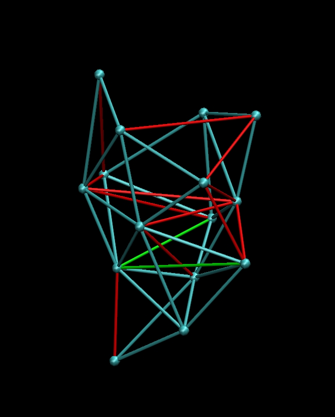
Then
rotate your molecule such that it is oriented as in the figures below
(you should recognize the pattern):
(click images to enlarge)
Then toggle the display of
molecule 0_rnap1.pdb
(in the VMD Molecule menu)
so that only the blue connectivities remain. Don't rotate the molecule.
Under the
'Mouse' menu select 'Add/Remove Bonds'. Remove any "red" bonds shown
above by clicking on both end points. Then add the "green" bonds the
same way. You should have a proper balance
between freedom of motion and stability of the skeleton. This takes
some experience, trial and error. The blue connectivities give a
reasonable fit that can be improved later. The edited
connectivity can then be saved into a PSF file from the VMD
command console (assuming your connectivity molecule
is still 'top'):
set sel
[atomselect top all]
$sel writepsf 6_rnap1.qpsf
|
Note: in run_tutorial.bash we copy 6_rnap1.qpsf from
the solution directory. This is a "cheat" that allows one to run the
entire script without waiting for this manual step. |
| LBG
Vector Quantization of the Low-Resolution Map
Now that the
skeleton connectivities have been
determined, the skeleton distances can be enforced with the local LBG
optimization algorithm of the quanvol
utility.
After entering
./quanvol
0_rnap2.situs 5_rnap1.qpdb
7_rnap2.qvol
|
the user is
prompted to enter
the density cutoff value. We enter the approximate surface threshold,
50. The start vectors are taken
from file 5_rnap1.qpdb and the user has the choice
optimization with LBG (enter 1) and of assigning vector distances. We
read them from the file 6_rnap1.qpsf
(option 3). Finally, the user is asked whether
nearest-neighbor connectivities should be learnt, we don't need this
option at the moment (enter 1). The file 7_rnap2.qvol
now contains the newly placed codebook vectors with the
distance
constraints enforced. As an exercise you should load both this file and
6_rnap1.qpsf,
together with 0_rnap2.situs into VMD:
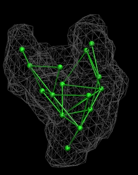
(click image to enlarge)
Below is the
output of the entire
quanvol LBG calculation. LBG is an iterative "gradient descent" method
that converges slowly, whereas
TRN (without the second argument as start vectors) uses a prespecified
number of calculations. The additional SHAKE statements
describe the convergence of the distance constraints:
./quanvol
0_rnap2.situs 5_rnap1.qpdb 7_rnap2.qvol
lib_vio> Situs formatted map file 0_rnap2.situs -
Header information:
lib_vio> Columns, rows, and sections: x=1-44, y=1-47, z=1-45
lib_vio> 3D coordinates of first voxel (1,1,1):
(140.000000,12.000000,0.000000)
lib_vio> Voxel size in Angstrom: 4.000000
lib_vio> Reading density data...
lib_vio> Volumetric data read from file 0_rnap2.situs
quanvol> Density values below a user-defined cutoff value will
not
be considered
quanvol> Do you want to inspect the input density values before
entering the cutoff value?
quanvol> Choose one of the following three options -
quanvol> 1: No
(continue)
quanvol> 2:
Show me the minimum and
maximum density values only
quanvol> 3:
Show me the voxel histogram
quanvol> 1
quanvol> Now enter the cutoff density value: 50
quanvol> Cutting off density values < 50.000000,
remaining
occupied volume: 10005 voxels (6.403200e+05 Angstrom^3)
lib_pio> 15 atoms read.
quanvol> Do you want to optimize the start vectors or skip and
proceed to the connectivity analysis?
quanvol> Choose one of the following two options -
quanvol> 1:
Optimize start vectors
with LBG
quanvol> 2:
Skip and proceed directly
to connectivity analysis
quanvol> 1
quanvol>
quanvol> Using start vectors from file 5_rnap1.qpdb.
quanvol>
quanvol> Vector distance constraints restrict undesired degrees
of
freedom.
quanvol> Do you want to add distance constraints?
quanvol> Choose one of the following three options -
quanvol> 1: No
quanvol> 2:
Yes. I want to enter them
manually
quanvol> 3:
Yes. I want to read
connectivities from a file and use start vector distances
quanvol> 4:
Yes. I want to read them
from a Situs constraints file
quanvol> 3
quanvol> Enter filename: 6_rnap1.qpsf
quanvol> 30 connectivities read from file 6_rnap1.qpsf
quanvol> The corresponding distances were assigned from file
5_rnap1.quanpdb
quanvol> Distance preconditioning step 1 -- 48 SHAKE distance
iterations
quanvol> Distance preconditioning step 2 -- 39 SHAKE distance
iterations
quanvol> Distance preconditioning step 3 -- 37 SHAKE distance
iterations
quanvol> Distance preconditioning step 4 -- 40 SHAKE distance
iterations
quanvol> Distance preconditioning step 5 -- 39 SHAKE distance
iterations
quanvol> Distance preconditioning step 6 -- 37 SHAKE distance
iterations
quanvol> Distance preconditioning step 7 -- 35 SHAKE distance
iterations
quanvol> Distance preconditioning step 8 -- 34 SHAKE distance
iterations
quanvol> Distance preconditioning step 9 -- 33 SHAKE distance
iterations
quanvol> Distance preconditioning step 10 -- 33 SHAKE distance
iterations
quanvol> Starting standard LBG vector quantization.
quanvol> It. 1 -- 53 SHAKE distance iterations
quanvol> It. 1 -- Average vector update: 6.108390e-01 Angstrom
quanvol> It. 2 -- 48 SHAKE distance iterations
quanvol> It. 2 -- Average vector update: 5.948577e-01 Angstrom
quanvol> It. 3 -- 48 SHAKE distance iterations
quanvol> It. 3 -- Average vector update: 5.773613e-01 Angstrom
quanvol> It. 4 -- 49 SHAKE distance iterations
quanvol> It. 4 -- Average vector update: 5.605641e-01 Angstrom
quanvol> It. 5 -- 52 SHAKE distance iterations
quanvol> It. 5 -- Average vector update: 5.440111e-01 Angstrom
...
quanvol> It. 118 -- 89 SHAKE distance iterations
quanvol> It. 118 -- Average vector update: 1.105221e-02 Angstrom
quanvol> It. 119 -- 89 SHAKE distance iterations
quanvol> It. 119 -- Average vector update: 9.938773e-03 Angstrom
quanvol>
quanvol> Final clustering -- 71 SHAKE distance iterations
quanvol> Final clustering -- Average vector update: 2.273772e-03
Angstrom
quanvol> Final clustering -- 71 SHAKE distance iterations
quanvol> Final clustering -- Average vector update: 2.607668e-07
Angstrom
quanvol>
quanvol> Codebook vectors have been written to file 7_rnap2.qvol
quanvol> The PDB B-factor field contains the equivalent
spherical
radii
quanvol> of the corresponding Voronoi cells (in Angstrom).
quanvol> Radius of gyration of the 15 codebook vectors: 42.462
Angstrom
quanvol>
quanvol> Do you want to update or save the input connectivities?
quanvol> Choose one of the following options -
quanvol> 1:
No. I'm done
quanvol> 2:
Update and save to a PSF
file
quanvol> 3:
Update and save to a
constraints file
quanvol> 4:
Update and save to both
PSF and constraints files
quanvol> 5:
Just save (don't update)
to a PSF file
quanvol> 1
quanvol> Bye bye!
|
|
Flexible,
Skeleton-Based Docking with Interpolation
As in the actin case above,
the
flexible docking is performed here in an approximative way by
interpolation from the 15 pairs of codebook vectors.
To
start the qplasty
optimization,
enter at the shell prompt
| ./qplasty
0_rnap1.pdb
5_rnap1.qpdb 7_rnap2.qvol 8_flexed_rnap.pdb |
The
flexed
structure will be written
to the file 8_flexed_rnap.pdb.
|
Visualization (RNA Polymerase)
The following sequence of
commands
in the VMD text console (cf. VMD
user guide) will load the original and flexibly docked rnap
structures, 0_rnap1.pdb (red) and 8_flexed_rnap.pdb (green), and
render them in colored tube representation. The script also renders the
target density map 0_rnap2.situs in gray:
mol
load
pdb 8_flexed_rnap.pdb
mol load
pdb 0_rnap1.pdb
mol load
situs 0_rnap2.situs
mol top 0
rotate
stop
display
resetview
display
projection orthographic
mol
modstyle
0 0 Tube 0.3 6
mol
modstyle
0 1 Tube 0.3 6
mol
modstyle
0 2 Isosurface 50 0 0 1 2 1
mol
modcolor 0 0 ColorID 7
mol
modcolor 0 1 ColorID 1
mol
modcolor 0 2 ColorID 2
|
Don't forget to hit "enter"
after the last line! The
final result
should look like this:
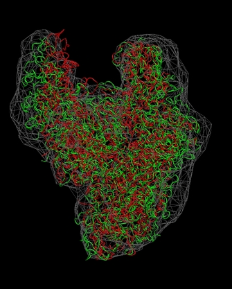
(click
image to
enlarge)
Note
that some density regions are not optimally filled by the flexed
structure. As an exercise, you can manually edit the connectivities or
codebook
vector positions to optimize the fit.
|
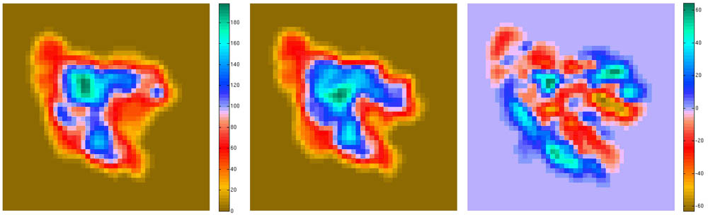
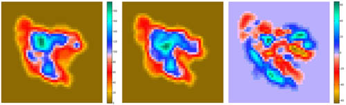
Visualization (2D Projections)
The
following script shows how to take advantage of bash shell scripting to
automate the work flow of rendering 2D projections and difference maps
between a structure and a density map.
Projections of
Difference maps = Difference of Projections (since there are no Situs
tools for the latter, we use the former approach):
# create
15A resolution map from 0_rnap1.pdb
./pdb2vol 0_rnap1.pdb tmp.situs <<< '2
1
4
-15
1
1
1
'
# match size of tmp.situs to that of 0_rnap2.situs
rm 9_rnap1_15.situs
./voledit tmp.situs <<< '1
0
5
0
1
1
1
0
0
0
4
2
45
1
47
2
46
0
12
9_rnap1_15.situs
0
13
'
rm tmp.situs
# create Y projection from 9_rnap1_15.situs
rm 9_rnap1_15.dat
./voledit 9_rnap1_15.situs <<< '2
-999
0
11
3
9_rnap1_15.dat
0
13
'
# create Y projection from 0_rnap2.situs
rm 9_rnap2.dat
./voledit 0_rnap2.situs <<< '2
-999
0
11
3
9_rnap2.dat
0
13
'
# create difference map
./voldiff 0_rnap2.situs 9_rnap1_15.situs 9_diff.situs
# create Y projection from 9_diff.situs
rm 9_diff.dat
./voledit 9_diff.situs <<< '2
-999
0
11
3
9_diff.dat
0
13
'
|
The
resulting projections (.dat files) can be inspected with a plotting
program such as MATLAB. The
final result
should look like this:
(click
image to
enlarge)
This script is part of
the included run_tutorial.bash script (see the file for detailed
documentation).
|
| Return
to the front page . |
|