|
User Guide
|
| This
guide is
intended to be
used as a reference manual. You may also want to follow the simple
steps
described in the tutorials
which give usage
examples
of the most important utilities. More documentation is also available
on
the methodology page
and in the published
articles . |
|
Content:
collage -
Simultaneous Multi-Fragment Refinement
colores - Exhaustive
One-At-A-Time 6D Search
ddforge - Flexible
Refinement Using Damped Dynamics.
elconde - Constrained
Deconvolution of Tomographic Filament Bundles
eul2pdb
- Graphical Representation of Euler Angles
map2map -
Format Conversion
matchpt
- Point Cloud Matching
pdb2sax
- Create a Simulated SAXS Bead Model from a PDB
pdb2vol
- Create a Volumetric Map from a PDB
pdbsymm
- Symmetry Builder
qplasty
- Interpolation of Sparsely Sampled Displacements
quanpdb
- Vector
Quantization of a PDB
quanvol
- Vector
Quantization of Volumetric Map
spatrac - Spaghetti Tracer
for Tomographic Filament Bundles
strwtrc
- Struwwel Tracer for
Tomographic Filament Networks
vol2pdb
- Create
a PDB from a
Volumetric Map
volaver
- Map Averaging
voldiff
- Discrepancy / Difference Mapping
voledit
- Inspecting
2D Sections and Editing of 3D Maps
volfltr
- Denoising 3D Maps and 2D Image Stacks
volhist
- Inspecting and Shifting the Voxel Histogram
volmult
- Map / Mask Multiplication
voltrac
- Alpha-Helix Detection and (Legacy) Filament Tracing
Header
File
and Library Routines
|
collage
- Simultaneous Multi-Fragment Refinement
Former name: colacor
Purpose:
collage performs
an off-lattice Powell optimization that refines a
single structure or a multi-fragment model (consisting of n
input PDB files) to the nearest maximum of the
cross-correlation score. The needed start model of fragments can be
built by eye in a graphics program, or based on colores or matchpt solutions. Due
to the large basins of attraction of each peak of the cross-correlation
score, the program is quite tolerant of initial orientational or
translational mismatches, and it is used without the colores-style
exhaustive search and peak search steps. The simultaneous
multi-fragment optimization of 6n
rigid body degrees of freedom is advantageous because the fragments see
each other and steric clashes are thus avoided by means of the
normalization of the cross-correlation. For more information see
(Birmanns
et al., 2011).
As an additional useful
option, collage can be used to report the
cross-correlation coefficient
between a density map and aligned atomic structure(s) without any fitting
performed.
Basic
usage
(at shell prompt):
| ./collage <Density
map> <PDB file(s)> -res
<float>
-cutoff <float> |
The basic
input parameters
are:
<Density
map> Density map in Situs
or CCP4/MRC format (auto detect). To
convert other maps to either of these formats use the map2map
utility.
<PDB
file(s)>
A single or few input PDB files can be specified as a sequential list
(all arguments are white space delimited, i.e. there should be no
commas
or other symbols between file names). To
avoid very long arguments when processing a large number of
input
files one can also specify a directory name as the second
argument. The designated directory should contain only relevant PDB
input structures
(identified by a .pdb or .PDB filename extension).
-res
<float>
Estimated resolution of the density map in Å.
[default
-res 15.0]
-cutoff
<float> Density map threshold value. All density levels
below
this
value
are ignored. You can use volhist
to
rescale
or shift the density levels in the voxel
histogram. [default -cutoff 0.0]
-corr
<int> This
option
controls the fitting
criterion.
Two
options
are implemented:
-corr
0
Standard
linear cross-correlation. The scalar product
between
the density maps of the low resolution map and the low-pass filtered
atomic
structure. This is the recommended criterion for high to medium resolution (<10Å) density maps
or for multi-fragment docking at all resolution levels. [default]
-corr
1
A Laplacian filter is applied by default to maximize
the
fitting
contrast. This is the recommended docking criterion
for single fragments docked to very low resolution (>10Å)
density maps. To
provide for a more robust algorithm when dealing with cropped
or thresholded maps, we implemented also a mask that filters out hard artificial
surfaces. Due to the masking and filtering expect overall smaller
correlation
values compared to -corr 0.
More
advanced
options (at shell prompt):
<-ani <float> Defines the resolution
anisotropy
factor (z direction vs. x,y
plane)
[default: -ani 1.0]. Allows
one to set a different resolution in the z direction vs. the x,y plane.
E.g. "-ani 1.5 -res 20" specifies a 30 A resolution in the z direction,
and a 20 A resolution in x,y. This is useful for researchers dealing
with
membrane protein or tomography reconstructions that have a reduced
resolution
in the z direction.
-nopowell
This flag skips the structure alignment using Powell optimization. Only the cross-correlation
coefficient of the input PDB file(s) is computed. By default the Powell optimization is turned
on.
-pwti
<float int> Powell tolerance and max number of iterations
of
the
Powell algorithm. This two parameters control the convergence of the
optimization.
By default the tolerance is set to 1e-6 and the max iterations are
limited
to 50.
-pwdr
<float
float> Initial gradient of the translational and rotational
search
in the
Powell optimization. By default the initial rotational gradient is set
to
3.5 degrees. The rotational gradient cannot be larger than 10 degrees.
If a larger value is chosen, that value is ignored and the gradient is
set to 10 degrees. The translational initial gradient is set to 25% of
the voxel spacing. To use the default value only for
the rotational or
only for the translational gradient, choose a negative number for the
parameter that must be left at default, and your chosen value for the
other.
-pwcorr
<int> This option sets the
Powell correlation algorithm. By default, the fastest algorithm which
reproduces the standard cross correlation coefficient to within the
Powell tolerance is determined at runtime.
-pwcorr
0 Determined at runtime [default]
-pwcorr 1 Standard
three-step code
-pwcorr
2 Three-step code with mask applied
-pwcorr
3 One-step code optimized for a single, small PDB
-boost <int float
float> Steric exclusion option (0=scale; 1=power), boost
threshold t,
and scale factor or exponent u.
In
multi-fragment fitting, overlapping subunits lead to enhanced densities
in the overlap region that reduce correlation values with the target
map. This penalty can be increased by applying a scale factor or power
law to high densities resulting from steric overlap. The threshold
parameter t
defines the fraction (typically < 1) of the maximum
single-subunit density at
which the boost kicks in. Densities above this threshold are increased
either by simple scaling (option 0): f(x>t) = ux, or by a power
function (option 1) which is continuously differentiable at the
threshold: f(x) =
x^u (t=0),
f(x>t) = (t-t/u)
+ (t/u)
(x/t)^u (t>0).
In practice thresholds near 0.9 and factors of 2-5, or
exponents of 5-20, seem
to
work
fine. Note that the density transformation affects only the upper tail
of the density distribution, i.e. non-overlapping regions are largely
unaffected. [default: none]
Input
at
program prompt:
None.
Output:
Shell
window: The cross-correlation
coefficient and other useful information about the progress of the
refinement. Depending on the overlap of structure and map, a good fit
with
-corr 1 (default Laplacian filter) setting may have values upto 0.5,
and with -corr 0 (standard correlation) may have values upto 0.9. These
values are smaller if the structures do not account for the entire map
density.
Files:
cge_001.pdb
... cge_00n.pdb The
atomic coordinates in PDB format of the final fits for each input
fragment.
cge_powell.log
This
file contains information about the 6n dimensional
Powell off-lattice search. Rotational
and
translational coordinates correspond to the first 6
columns, the Euler angles are in degrees.
|
| colores
- Exhaustive One-At-A-Time 6D Search
Purpose:
colores
is a general purpose, multi-processor
capable rigid-body
search
tool, suitable for one-at-a-time fitting of single subunit structures,
which are not necessarily
expected to account for the full map. The fitting procedure consists of
three separate steps: (A) An exhaustive rigid body search on a discrete
6D lattice (3
translational
and 3 rotational degrees of freedom);
(B) an automatic ("black box") peak detection based on the correlation
scores on the lattice (returning a set number of solutions); (C) the
final off-lattice refinement of solutions to the nearest maximum of the
correlation score (similar to collage). For low-resolution density maps, an optional Laplacian-style filter can be turned on that increases the fitting
contrast by enhancing molecular shape contours (for more info see the corresponding
methods page and Chacón and
Wriggers,
2002).
One
can balance the precision of the
search (angular granularity, option -deg, and translational
granularity=voxel spacing of map) with the compute expense. However,
please consider
first the relationship of procedures (A-C) and the granularity step
sizes.
The translational search
in (A) is
FFT-accelerated, whereas the rotational search is performed by
evaluating a list of Euler angles for each voxel. In
recent years a number of colores clones have been developed by us and
other groups that aim to accelerate the search in (A) further, but the
refinements in step (C) cannot be FFT-accelerated and our
tests showed that for most practical purposes the current
implementation of (A) is efficient enough to shift the performance
bottleneck to steps (B) and (C).
The standard translational granularity (voxel spacing of EM map sampled
at Nyquist rate) and the recommended rotational granularity (20-30°)
are well within the large basin of attraction of the refinement in (C),
so finer granularity is not normally needed. The proposed relatively
coarse sampling in (A) also has the benefit of providing more
spread-out solutions in step (B), resulting in fewer redundant runs in
(C). Therefore, a default -deg rotational step size of 30°
degrees is provided, and a translational down-sampling is performed,
when necessary, to match the voxel spacing to the map resolution
according to Nyquist rate (this is a sanity check that prevents
absurdly small translational steps, e.g. in maps created by pdb2vol).
There
is no reliable way to validate the accuracy of the fitted models based
on the precision of the fitting alone (shape of peaks, scoring values
etc) as
was pointed out by Henderson
et al., 2012.
We believe that models are best validated in a comprehensive test that
includes independent biological information. As an inspiration for how
this is done for colores see the supplementary
material of a user paper we recommend: Tung
et al., 2010, doi:10.1038/nature09471.
Basic usage
(at shell prompt):
./colores <density
map> <PDB
structure> -res <float>
-cutoff <float> -deg <float> -nprocs
<int>
|
The basic
input parameters
are:
<density
map> Density
map in Situs or CCP4/MRC format
(auto detect). To
convert other maps to either of these formats use the map2map
utility.
<PDB
structure> Atomic structure in PDB format.
-nprocs
<int> This option sets the number of processors used for
the
on-lattice 6D search and the off-lattice Powell optimization. Colores
supports shared memory systems with multiple core and/or hyperthreaded
processors.
Usage on more than 16 cores may be unstable on
some systems, use larger numbers at your own risk. [default:
the number of logical cores of the CPU but no more than 16]
-res
<float>
Estimated resolution of your density map in Å.
[default
-res 15.0]
-cutoff
<float> Density map cutoff value. All density levels
below this
value
are set to zero. You can use volhist
to
rescale
the density levels or to shift the background peak in the voxel
histogram
to the origin. [default -cutoff 0.0]
-deg
<float> Angular sampling of the
rotational search space in
degrees.
For typical electron microscopy maps the recommended angular step size
is 20-30° (a
smaller step size might return near-redundant solutions in the peak
search, and any orientational mismatch will be refined in the
subsequent Powell optimization anyway). [default -deg 30.0]
-corr
<int> This
option controls the fitting
criterion.
Two
options are implemented:
-corr
0 [default
for res.<10Å]
Standard
linear cross-correlation. The scalar product
between
the density maps of the density map and the low-pass filtered
atomic
structure.
-corr
1 [default for res.>=10Å] A
Laplacian filter can be applied to maximize
the
fitting
contrast in the case of low-resolution density maps (useful from about 10 to 25Å resolution). To
provide for a more robust algorithm when dealing with cropped
or thresholded experimental
data, we implemented a mask that filters out hard artificial
surfaces. Due to the masking and filtering expect overall smaller
correlation
values compared to -corr 0. Also, due to the emphasis on contour
matching over interior volume matching some solutions may not be fully
contained within the map if the subunit surfaces are large compared to
the volume.
More
advanced
options (at shell prompt):
-ani
<float>
Defines the resolution anisotropy
factor (z direction vs. x,y
plane)
[default: -ani 1.0]. Allows
one to set a different resolution in the z direction vs. the x,y plane.
E.g. "-ani 1.5 -res 20" specifies a 30 A resolution in the z direction,
and a 20 A resolution in x,y. This is useful for researchers dealing
with
membrane protein or tomography reconstructions that have a reduced
resolution
in the z direction.
-erang
<float float float float float float>
Defines the rotational space limits according to the range of the Euler
angles (psi, theta, phi). By default the entire rotational space is
considered
[default: -erang 0 360 0 180 0 360]. Note that the Euler
angle
range
is not limited to these standard intervals, so you can specify also
negative
values (within certain limits), but in any event any colores output
angles
are remapped to the standard intervals. For example, if you want to
perform
a fine search of 2° angular sampling in only one of the Euler
angles,
these are the options:
| ./colores
em.sit
atoms.pdb
-res 9.0 -cutoff 1.0 -deg 2 -erang 0 360 0 0 0 0 |
-euler
<int> There are three ways to generate an exhaustive
list of Euler
angles that covers (nearly) uniformly the rotational space for a given
angular sampling
(option -deg). The proportional method yields very even
results and also performs well for smaller intervals specified via
'-erang'. The pole sparsing method is widely used but yields slightly
less
uniform distributions. The spiral method also produces a less uniform
distribution, but for medium
to low resolution docking it is quite reasonable. The Euler angles are
saved to a file col_eulers.dat, and you can edit this file and reload
it
using the -euler 3 option. This way, you can also load any manually
generated
Euler angle files.
-euler
0 Proportional method [default]
-euler
1
Pole sparsing method
-euler 2 Spiral method
-euler 3
<filename> Input file
Here is
an example generating the Euler angle distribution with 8°
angular
sampling using the spiral method:
./colores
em.sit
atoms.pdb
-res 9.0 -cutoff 1.0 -deg 8 -euler 2
|
-peak
<int> This option sets the peak search algorithm. By
default, a combined sorting and filtering-based approach is used. A
stand-alone filtering-based algorithm is available as an option.
-peak
0 Original peak search by sort and filter [default]
-peak 1 Peak search by
filter only
-explor
<int> Controls the number of the best fits found in the
6D
on-lattice
search to be subsequently refined by Powell optimization. This number
is only an upper bound for the final number, since redundant solutions
are removed in the Powell stage. [default -explor 10]
-sizef
<float> FFT zero padding factor. The low resolution map
is
enlarged by a margin of
width sizef times
the map dimensions. We have optimized the zero padding empirically [default
-sizef 0.1 for standard and 0.2 for Laplacian correlation]
-sculptor
Save
additional output files for interactive
exploration (manual peak
search) with our Sculptor
molecular graphics program. This is documented in a
Sculptor tutorial under item “Loading exhaustive search data
into Sculptor“ [default: Off]
-nopowell
This flag skips the Powell optimization and only the on-lattice search
is performed. By default the Powell optimization is turned on.
-pwti
<float int> Powell tolerance and max number of iterations
of
the
Powell algorithm. This two parameters control the convergence of the
optimization.
By default, the tolerance is set to 1e-6 and the max iterations are
limited
to 25.
-pwdr
<float
float> Initial gradient of the translational and rotational
search
in the
Powell optimization. By default the initial rotational gradient is set
to
25% of the angular sampling (but not larger than 10°), and the
translational
initial gradient is set to 25% of the voxel spacing. To use the default
value only for the rotational or only for the translational gradient,
choose a negative number for the parameter that must be left at
default, and your chosen value for the other.
-pwcorr
<int> This option sets the
Powell correlation algorithm. By default, the fastest algorithm which
reproduces the standard cross correlation coefficient to within the
Powell tolerance is determined at runtime.
-pwcorr
0 Determined at runtime [default]
-pwcorr 1 Standard
three-step code
-pwcorr
2 Three-step code with mask applied
-pwcorr
3 One-step code for small probe
structures
-nopeaksharp
This flag skips the peak sharpness estimation procedure in order to
save processing time. By default, the peak sharpness estimation is
turned on.
Input
at
program prompt:
None.
Output:
Here is a
brief description
of the output files (see also the file headers);
col_best*.pdb
The atomic coordinates in PDB format of the best fits found in the
search.
The total number of best fits saved is controlled by the option
-explor,
but only non-degenerate fits are returned, so the number may be smaller
than specified by the -explor option. The PDB header contains
information
about the docking (sampling, fit criteria used, correlation values,
position
and orientation etc.). It also includes a table containing the angular
variability of the correlation about the fit.
col_rotate.log This
file contains the best translational fit (on-lattice) found for each
rotation.
The first 3 columns are the Euler angles (in degrees), the next 3
columns
are the translational coordinates that gave the highest correlation
value,
followed by the correlation value (not normalized).
col_powell.log
This
file contains information about the Powell off-lattice search performed
for the best fits from 6D lattice search. As before, rotational
and
translational coordinates correspond to the first 6 columns , but note
that the Euler angles are in radian units.
col_trans.sit
The on-lattice translation function (in Situs map format). Since the
translational
search space corresponds to the input map lattice , we can generate a
map
in which density values are the correlation values normalized by the
maximum. You can use map2map
to
convert this to
other formats.
col_trans.log
Same as col_trans.sit, but instead of a map, the translational
correlation
values are stored in a regular file. Each row that corresponds to a
lattice
coordinate (columns 4,5,6) shows the corresponding Euler angles
(columns
1,2,3) in degrees that exhibit the highest correlation value (column
7).
col_eulers.dat
This file contains the list of uniform Euler angle triplets that
defines
the rotational space search. You can load such a file by using the
option
-euler 3. You can also inspect this file with the eul2pdb
tool.
col_lo_fil.sit
The zero padded, interpolated, and filtered target volume in Situs
format just prior
to correlation calculation. This map is useful mainly for inspecting
the effect of low-pass or Laplacian filtering. You
can use map2map
to
convert this to
other formats.
col_hi_fil.sit
The filtered (and centered) probe structure on the lattice in Situs
format just prior
to correlation calculation. This map is useful mainly for inspecting
the effect of
low-pass or Laplacian
filtering. You
can use map2map
to
convert this to
other formats.
Additional output files will be written for interactive
exploration
with the -sculptor
option (see
colores output and the Sculptor
documentation).
Notes:
- Depending
on the overlap of structure and map, one can expect correlation values
of about 0.6-0.9 or 0.3-0.5 for standard and Laplacian correlation,
respectively. These guideline numbers would be
smaller if the fitted atomic structure does not account for the entire
map density.
- The time
estimation gives
a quite accurate estimate of the on-lattice 6D search time, however,
the
subsequent peak search and off-lattice Powell optimization are not
considered in the
estimation
and depend on the -explor number. You could save time
if you use only the carbon alpha or backbone atoms of the input
structure but the savings are often insignificant so we recommend
fitting with all heavy (non-hydrogen) atoms.
- If you have a large map you can try to crop
the
data
to a region of interest (e.g. the asymmetric unit). Allow for
sufficient
room for the probe structure since you do not know its exact location a
priori.
- This
is a rigid body
search. If you expect large, induced fit conformational changes, you
can
dissect your atomic structures into rigid-body domains and perform the
docking
with each of them individually. Alternatively, you may want to try our flexible
fitting strategies.
|
| ddforge
- Flexible Refinement Using Damped Dynamics.
Purpose:
ddforge
is a tool for performing flexible fitting and refinement of atomic
models against medium resolution density maps. It works in generalized
coordinates (positional and internal coordinates) and, instead of
harmonic potentials, it uses dampers (“shock absorbers”) between pairs
of atoms to preserve the structural integrity of the molecule. Details
of the method can be found in the paper (Kovacs,
Galkin and Wriggers, 2018).
Usage (at
shell prompt):
Type
1: PDB to be fitted
in density map:
|
./ddforge
<PDB> <density map> <min disp
between
outputs> <map resolution> <density
threshold> <damp/drag ratio> <side-chain
optim> <force-field
cutoff distance> <max disp per step> [-rdfile
<residue data>] [-dcfile
<distance constraints>]
|
Type
2: PDB1
to be flexed toward PDB2:
|
./ddforge <PDB1>
<PDB2> <min disp
between outputs> <damp/drag
ratio> <side-chain
optim> <force-field cutoff distance> <max
disp per step> [-rdfile <residue data>] [-dcfile <distance
constraints>]
|
Type
3: PDB1
to be flexed toward PDB2 and fitted
in density map:
|
./ddforge <PDB1>
<PDB2> <density map> <min disp
between
outputs> <map resolution> <density
threshold> <damp/drag ratio> <side-chain
optim> <force-field
cutoff distance> <max disp per step> [-rdfile <residue data>]
[-dcfile
<distance constraints>]
|
Mandatory arguments (to be
given in this order):
<PDB>
or <PDB1>
<PDB2>
Atomic
structures in PDB format (extension “.pdb”).
<density
map> Density
map in Situs
or CCP4/MRC format
(auto detect). To
convert other maps to either of these formats use the map2map
utility.
<min
disp between outputs> Desired minimum RMS
displacement between
output conformations, in Å. Typical range: 0.5 - 5.
<map
resolution> in Å.
<density
threshold> Density values below
this will be set to 0, and all others will be lowered by this amount.
<damp/drag
ratio> Ratio between
damping and drag strengths. Typical range: 10-100.
<side-chain
optim>
Side-chain
"optimization" flag. This enables the rebuild of full atomic side
chains from the truncated ones used internally by ddforge (see Figure
below). Possible values: 0: no side-chain rebuild; 1:
initial rebuild only; 2: subsequent only (only new
conformations
will be treated); 3: both. For options 1, 2 and 3, you need to download SCWRL4
and install it (in order for ddforge to find
the executable "Scwrl4", you
can put it in the folder requested by ddforge and denoted in
ddforge.c line 2727 (or to specify your own path, edit this
line
in the code and and reinstall
ddforge). Also, after installing
SCWRL4, you may also need to edit the Scwrl4.ini
file so the line at the top "[RotLib] FilePath" points to your side
chain library location. Please note that ddforge behavior is slightly
modified by the option flag. For options 1 and 3, SCWRL4
will automatically remove any unknown molecules or non-amino
acid
residues from the PDB, which may be unintentional. If you run your
model the first time it is better to use options 0 or 2, in
that
case ddforge will terminate with an error message if it finds unknown
residues and you can fix these issues manually in your PDB.
<force-field
cutoff distance> Maximum distance
in
Å for the action of the force field [which attracts the
PDB toward the
target(s)
(PDB and/or map)]. Typical range: 10-50.
<max disp per step>
Maximum allowed RMS displacement of the PDB
at each step of the integration, in Å. Typical range: 0.5 - 2.
Optional arguments:
-rdfile <residue
data> Residue data file
name. See detailed description below.
-dcfile <distance
constraints> To impose distance
constraints, a file with
their definition can be specified as the last argument. See detailed
description
below.
Input at
program prompt:
None.
Output:
A
series of PDB files is created, with
names built from the name of the PDB1 file, by adding “.deform.n”
to its base name, for n
ranging from 1
to the total number of conformations produced till convergence. These files describe the
trajectory undergone
by the initial atomic structure until its final fitted conformation. Also, there is output sent
by default to the
“stdout”
stream. This can be redirected to a text file.
First,
ddforge echoes the parameters
specified on the command line, and basic information about the input
files.
Then there is a progress log of the optimization of sigma and threshold
parameters used for generating the simulated maps. Then comes the
evolution
proper. The first
column, “Conf#”, gives
the conformation number of the PDB structure written to file at that
time.
“Step#” refers to the time step in the integration procedure. “Time” and “speed” are
simulation values —not
really useful for the user. “Disp.” refers to the RMS displacement of
the
structure at that step. “Dist_cut” is the cutoff distance for
connecting pairs
of atoms with dampers. “Overlap”
is the
amount of overlap between the density map and the simulated map, which
can be used
as a measure of convergence. “Cos”
is an
internal parameter used in time-step control —not relevant to the user. Lastly, “Compute time” is
the actual CPU time
up to that point of the trajectory.
The
program will stop automatically according to a convergence criterion
based on the analysis of the overlap evolution over time. The criterion
aims at recognizing the saturation of the overlap function, by means of
an exponential regression. Details about this are given in the paper.
Note that the program will need to run slightly past this point to
estimate the regression parameters. When it eventually stops,
the screen output will indicate the proposed safe ending time, and we
recommend to use the conformation just prior to this time, as the later
conformations (used for regression) will probably be over-fitted.
Optional residue data file:
This allows the user to
fine-tune the modeling of the amino acid
resides. If this
file is not
specified on the command line, ddforge will assume that all atoms are
freely movable and that all internal degrees of freedom
are free.
The structure of this
optional residue data file is exemplified here:
CODE CH.ORI.
RES.ORI.
CH.TAR.
RES.TAR.
31
A
57
A
5
28
A
58
A
6
28
A
59
A
7
28
A
60
28
A
61
28
A
62
A
10
28
A
63
A
11
where
CH = PDB chain character, RES = PDB residue number, ORI = origin, TAR =
target.
The
first line is
ignored by ddforge, it can
be used for comments, or as a
header indicating the name of each column. Starting with line 2, every
line holds a separate residue specification. Residues are identified by their PDB residue
number and by the PDB chain
character, as present in the origin PDB file. Columns
4 and 5 ("target"
residues) are
only needed for Type 2 or 3 usage (i.e. fitting to another PDB, see
below).
The
CODE column is a decimal code number that specifies
which variables of each residue
(of the “origin”
structure) are to be free, and whether the residue should be static
(fixed) in
space or
not (this is useful for “loop closures”).
This is indicated after transforming the
decimal code into binary form. The resulting bits and their decimal
weights (powers of 2) have the following meaning:
Bit Weight
Meaning
0*
1
(x,y,z) free
1*
2
(lambda,theta)
free
2
4
phi
free
3
8
psi
free
4
16
chi
free
5
32
(unused
at this time)
6
64
backbone
atoms static
7
128
(unused
at this time)
* apply
only
to the first residue
of each chain
Please
refer to the figure below for the meaning of the variables. The user should note that ddforge uses a
hierarchical, internal coordinate system for each independent chain.
The global (absolute) position and orientation of the entire chain is
set by the x, y, z coordinates of the first N(1) atom, as well as by
the lambda, theta, and phi(1) angles (six rigid body degrees of
freedom). This is the reason why bits 0 and 1 apply only to the first
residue of each chain. All remaining degrees of freedom of the chain, designated by bits 2, 3, and 4, are internal angles.
Any
invalid codes are
automatically corrected. (For example, if bit 0 or bit 1 is set for a
residue
that's not
the first of the chain, or if bit 3 is set for the last residue of a
chain, or
if bit 2 is set for a proline residue if it’s not the first of the
chain, etc.)
Special
cases:
- In case the residue data file is not
specified on the command line, ddforge will assume that all
residues have a decimal code number of of 31, which means that x, y, z,
lambda, theta, phi, psi, and chi are all free.
- In
case the residue data file is used, but a
residue is
missing in the residue data file (although
present in the
origin PDB),
it is treated as if its
code were
0. The effect of this depends on whether the missing residue is (i) at
the start of the chain (the residue is static and the entire chain is
pinned down) or (ii) in the middle of the chain (the phi,psi,chi angles
are frozen, i.e the residue moves as a rigid body).
- If
there are gaps in the same chain, i.e. there are missing residues in
the origin PDB itself, we recommend assigning a new chain
character to every separate polypeptide chain segment. The program will
try to handle such gaps gracefully by assigning a very long rigid
"bond" between adjoining segments of the same chain (rigid, because
omega angles, i.e. torsions about C-N bonds, are taken as constants).
- Bit 6 is a special modification that allows to fix
only the backbone atoms during the refinement.
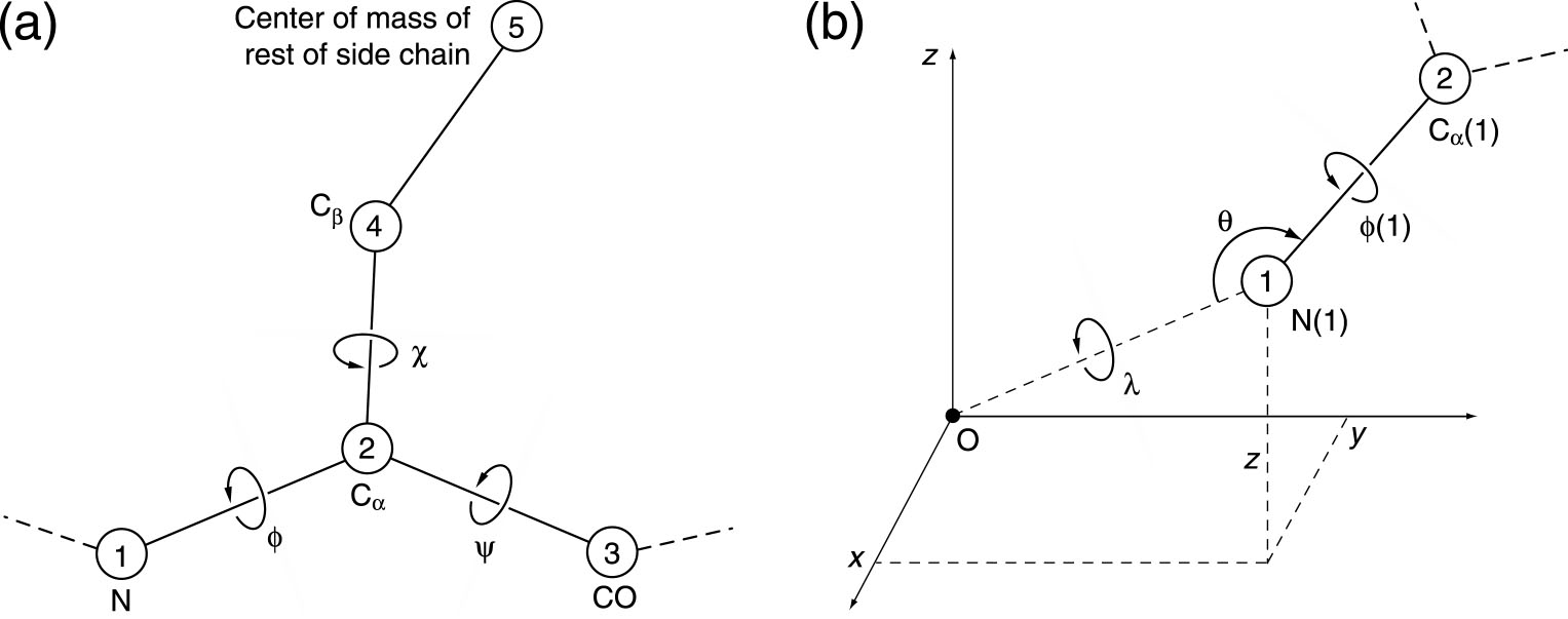
Figure: ddfforge
residue data file variable name conventions
Columns
4 and 5 (see above residue data file example) are needed only when an atomic
structure (i.e. PDB2) is
used as
the target; the columns indicate the target residue toward which the
origin residue of columns 2 and
3
should be pulled. In
the above example, the three
backbone atoms are pulled toward the corresponding atoms of the target
structure. As the
example shows, some
residues may be left without any target (no force is then exerted on
those
particular atoms).
Setting
up residue data files for large PDBs might become labor intensive. You
can find templates and scripts for generating them in the flexible fitting tutorial.
Optional distance constraints file:
The user has the option
to specify this
file to impose distance constraints between certain residues, e.g. for
purposes of keeping secondary structure elements intact during the
refinement. The structure of
this file is exemplified here (data
will be read from line 2, line 1 is
a user-defined header that will be ignored):
CH RES CH
RES
A 9
A
20
A 12
A
17
A 154 A
300
B 9
B
20
B 151
B
297
B 154
B
300
C 103
C
132
C 107
C
136
C 151
C
163
C 151
C
297
where
CH = chain and RES = residue. Each
line (after the first) represents one distance constraint
between the residues given. The first 2 columns refer to one of the
endpoints
of the constraint, while the last 2 columns refer to the other endpoint.
|
| elconde
- Constrained Deconvolution of Tomographic Filament Bundles
Purpose:
ElConDe (Electron tomogram
Constrained Deconvolution) can correct missing-wedge
artifacts in filamentous tomograms. It also denoises the data and
generates a file with the traced filaments. The deconvolution problem
is
recast as a constrained quadratic optimization problem, which is
handled by a dedicated solver. Details of the method can be found in
the paper ( Kovacs
et al., 2020).
We note that ElConDe interprets the entire map in terms of the filament
templates, so
there is a risk of false positives when applied to tomograms that
include non-filamentous features such as organelles and membranes.If
false positives are a concern, we recommend instead the image
processing tools strwtrc and spatrac, which were optimized to limit both false positives and false negatives. Also, ElConDe
works best when the filament directions closely follow a mean
direction, such as in tightly packed filament bundles of the shaft
region of stereocilia. Therefore, we recommend our strwtrc utility if you need to trace randomly oriented filament networks.
Usage
(at
shell prompt):
./elconde -opt n
<argument
list>
|
The argument “n” specifies
the operation to be carried out. The program should be called
sequentially with n = 0, 1, 2, and 3, see details below. Depending on
the data, some of
these steps may not be necessary.
n
= 0: Spatial decomposition of the input map into smaller maps:
Calling elconde with n = 0
will generate a set of smaller subtomograms that cover the input map.
We call the input map “global map” and the smaller maps “local maps”.
The local maps will overlap
with each other along their boundaries as a way to deal with boundary
artifacts. We recommend a size of roughly 1 million voxels for each of
the local maps, as a good compromise between memory requirements for
the solver and artifacts in the solution caused by wraparound effects
if the maps are too small. This ideal size is given in the parameter
file (described below), and the default values in there already satisfy
the above size recommendation.
elconde -opt 0
<infilename>
<parfilename> <outbasename>
|
Arguments
(mandatory):
<infilename>
(input) Global
tomogram map in Situs
or
CCP4/MRC format
(auto detect).
<parfilename>
(input) File with
user-supplied parameters (described below).
<outbasename>
(output) Base name
for local maps, i.e. first part of the name (chosen by the user) for
all the
local maps to be created. The remaining part will be appended
automatically as
a triplet of indices for each of the local maps (plus the suffix
“.situs”). These intermediate maps are
generated in text-based Situs
map format so they can be easily inspected.
n
= 1: Map deconvolution and local U-map generation:
Calling elconde with n = 1
will proceed to the deconvolution of all the local maps generated in
the previous step . This part (function condesa in the
source code) runs in parallel, using
OpenMP with
OMP_NUM_THREADS cores (or as many as available on the system if not
set). E.g.
export OMP_NUM_THREADS=4
will use 4 threads. This part also generates log files for each of the
maps, containing details on the progress of the optimization
iterations. Screen output is also produced. Both can be controlled by
parameters in the parameter file (described below).
./elconde -opt 1
<inbasename> <parfilename>
<Ubasename> [Tbasename]
|
Mandatory
arguments:
<inbasename>
(input) Base name of local maps. This should be the same as the outbasename of the previous step, n = 0.
<parfilename>
(input) File with user-supplied parameters (described below).
<Ubasename>
(output) Base name for the “U-maps”. These are coefficient maps (in text-based Situs
map format, so they can be easily inspected)
whose convolution with the “shape kernel” yields the deconvolved maps.
The U-maps will be combined together in the next step.
Optional
argument:
[Tbasename] (output)
Base name for the deconvolved maps. The user may choose not to have
these maps created, especially if they are many, as they may be large,
and are not needed if the next steps (n = 2 and 3) will be carried out.
n
= 2: Combination of the U-maps into a global U-list:
Calling elconde with n = 2
will collect (function collect
in the source code) all the U-maps generated in the previous step and
generate
a global “U-list”. This is a reduced representation of a U-map, which
covers the whole of the input (global) map. Its convolution with the
“shape kernel” yields the global deconvolved map (done in the next
step.
./elconde -opt 2
<Ubasename> <parfilename>
<Ufilename>
|
Arguments
(mandatory):
<Ubasename>
(input) Base name of local U-maps. This should be the same as the Ubasename of the previous step, n = 1.
<parfilename>
(input) File with user-supplied parameters (described below).
<Ufilename>
(output) Name for the global “U-list” file.
n
= 3: Tracing of the global map:
Calling elconde with n = 3
will use the U-list created in the previous step and generate a traces
file (UCSF Chimera .cmm format). The corresponding function in the
source code is named ctracer.
It will optionally create the global deconvolved
T (or "true") map described in
the paper (Kovacs
et al., 2020).
We observed that the T map
looks best for tightly packed (near-parallel) bundles of actin
filaments in the shaft region of stereocilia, but it was not as
well defined in semi-organized actin filaments in the taper region of
stereocilia. Therefore, the output of the T map is optional, whereas
the traces are considered more reliable.
elconde -opt 3
<Ufilename>
<parfilename> <Cfilename> [Tfilename]
|
Mandatory
arguments:
<Ufilename>
(input) Global U-list obtained in the previous step. This should be the same as the Ufilename of the previous step, n = 2.
<parfilename>
(input) File with user-supplied parameters (described below).
<Cfilename>
(output) Traces file (in UCSF Chimera .cmm format).
Optional
argument:
[Tfilename] (output) Global T ("true")
deconvolved map (MRC or Situs format, depending on .mrc, .sit or .situs
file name suffix).
Parameter
file (mandatory):
This
required configuration file contains all the parameters needed for the
deconvolution process. All steps above need to be run with the same
parameters. A self-explanatory and documented template file
"elconde_parameters_template.txt" can be found in the doc
folder
of the Situs distribution. The user should modify the parameter values
in this template according to their specific problem. The order of the
parameters in the file must not be altered. The procedural context for
the parameter choices can be found in
the paper (Kovacs
et al., 2020).
|
| eul2pdb
- Graphical
Representation of Euler Angles
Purpose:
The eul2pdb
utility is used to generate a graphical representation of a set of
Euler angles resulting from a colores
run. The eul2pdb programs writes a pseudo-atomic structure in a
PDB formatted file where the set of Euler angles is represented as a
set
of points on a 10A radius sphere. This file
can then be inspected with a visualization program (for example VMD).
Usage (at
shell prompt):
./eul2pdb col_eulers.dat
out_file
out_file: output file, PDB
format |
Input at
program prompt:
None.
Output:
Pseudo-atomic structure
in PDB-format. Each triplet of Euler angles in the input
file is represented as a point on a 10A radius sphere. The phi Euler
angle (rotation in the projection plane) is encoded in the B-factor
column of the PDB file (in radians units), whereas theta and psi
correspond to longitude and latitude on the sphere.
|
| map2map
- Format Conversion
Former names: convert,
conformat
Purpose:
Situs programs require
density maps either in Situs
or in CCP4/MRC format. The details and conventions of these
formats are documented elsewhere.
The
map2map program
converts other map formats to and from these supported formats.
The map2map
utility reads and writes many file
formats used by standard EM or crystallographic application software.
These include the
MRC,
SPIDER,
and CCP4 formats and generic 4-byte floating-point binary
formats
(automatic byte-order adjustment). X-PLOR maps in ASCII format, and
ASCII
files that contain a sequence of density values in free format are also
recognized. The reverse conversion to CCP4,
MRC,
X-PLOR, or SPIDER format is also supported.
Usage (at
shell prompt):
| ./map2map file1 file2
file1: inputfile
file2: outputfile
|
Interactive input at
program prompt (for automation see below):
- Input
file
format.
- Input
file
specific header fields if they are missing or if manual editing of
fields is selected.
Output:
Density file in
selected format.
If necessary, the program permutes the axis order (CCP4 and
MRC) and interpolates maps to a cubic lattice (X-PLOR,
CCP4,
MRC). Details vary by map format and are too numerous to
list
here, please read about the Situs and CCP4/MRC conventions here and inspect the program text in
the terminal window carefully.
Notes:
- Also
check
out the free conversion programs MAPMAN/RAVE,
and
especially em2em
which also has Situs and CCP4/MRC format options.
- The maps are quite
robust under
most round trip conversions, but note that
header fields
WIDTH,
ORIGX,
ORIGY, ORIGZ are not part of the
SPIDER
specification and cannot be saved in SPIDER.
- Advanced
users may try the manual assignment of header fields, if
available.
- You can automate
this interactive program by "overloading" the standard input (if you
put expected
values in a script, see run_tutorial.bash script in the tutorials).
|
| matchpt -
Point Cloud Matching
Supersedes former programs:
qdock, qrange
Purpose:
The
classic Situs 1.x style matchpt ("matchpoint") utility is a
command-line program for matching arbitrary sized 3D point sets
(coarse-grained models), which can be generated on the fly or by using the output of the Situs
programs quanpdb
and quanvol. matchpt
can dock a subunit into a larger target map, i.e find N codebook vectors
within another set
with M vectors, N<M (where M
≈ nr. units * N) and match them. To solve this problem, matchpt
uses a heuristic and investigates only a subset of all possible
permutations of feature-points (Birmanns
and Wriggers, 2007).
The idea of matching
point sets was based on the observation that for many low-resolution
maps numeric values of the
cross-correlation (CC) are often in a narrow range and less
discriminatory as the RMSD values of the feature point (Wriggers
et al, 1999).
This is due to the fact that feature points can reliably and
reproducibly encode the molecular shape even in the absence of interior
(secondary structure) density features. Therefore, it makes sense for
difficult low-resolution maps to try matchpt as an alternative to
the CC-based tools colores
and collage.
In the default mode a user would explore the quality of the match of
the
point clouds by minimizing their RMSD. Alternatively, the
minimum
of the statistical
variability (here: sum of average variabilities of both point sets) can
be used for selecting an optimum number N. M as it was found to be a
good estimator for the docking accuracy (Wriggers
and Birmanns, 2001).
Finally, a user may wish to explore the standard cross-correlation
(CC),
which is discretely sampled by the point cloud matches (however, as
stated CC refinement is not the main purpose of the program as
more powerful CC-based tools exist).
Basic usage (at
shell prompt):
./matchpt
file1 file2 file3 file4 [options]
file1:
inputfile 1,
Codebook
vectors from quanvol in PDB format
Use NONE if the codebook vectors should be calculated within matchpt.
In that case matchpt will compute and match a series of vector sets and
will return the result with the smallest rmsd. file3 also has to be set
to NONE.
file2:
inputfile 2, Density
map. Use NONE if no correlation calculation desired
file3:
inputfile 3, Codebook
vectors from
quanpdb in PDB format.
Use NONE if the codebook vectors should be calculated within matchpt
file4:
inputfile 4,
High-resolution
structure in PDB format. Use NONE if only the codebook vectors should
be matched.
|
Optional
command
line parameters:
-res
<float>
Estimated resolution of file2 in Å. This currently affects
only the
computed cross-corelation value, not the docking.
[default
15.0Å]
-explor
<int> Controls the maximum number of docking solutions
that are
'explored' and written
to disk. This number is an upper bound since the solutions must pass
the anchor point matching criteria below.
[default
10]
-mincv
<int> For autogeneration of
feature points, or "codebook vectors" (CV), minimum
number N of vectors per structure (file4)
unit,
must be >= 4. [default 4]
-maxcv
<int> For
autogeneration of codebook vectors, maximum
number N of vectors per structure (file4) unit,
must be >= mincv.
[default 9]
-units
<float> For
autogeneration of N
and M (M
≈ units * N) codebook
vectors, number
of structure units contained in target volume.
[default
1.0]
-nprocs
<int>
Number of parallel processing threads. This
is still an experimental feature, so use with caution: We noticed that
the parallel performance can be compiler or
machine-dependent. If
a
multi-threaded application appears slow or unstable on your system, we
recommend to reduce the number of threads, or use the default serial
application. [default:
1]
-anchor
<float> Radius of initial anchor point triangle
search
space in
Å. [default
12.0Å, the larger the slower]
-radius
<float> Radius of the
neighbor-search in
Å.
[default 10.0Å, the larger the slower]
-wildcards
<int> Wildcards: How many unmatched points are allowed.
To avoid
false positives, it should not be larger than 10% of N. [default
0, the
larger the slower]
-penalty
<float> Wildcard penalty in
Å.
How much should the solutions be penalized if they include unmatched
points. [default: 1Å]
-runs
<int>
Number of anchor point runs. The algorithm will try different anchor
point triangles
if set to > 1. [default:
3]
-cluster <int>
Number of statistically independent runs used in the
clustering of
the CV and in the determination of their variabilities. The CV and
their variabilities will become more accurate with larger number but
compute time increases linearly. [default:
8, the
larger the slower]
-ident
<float> Distance cutoff in
Å
for removing identical solutions. Useful mainly for oligomeric systems.
[default
0Å, the higher the more results are
filtered]
-ranking <int> Sets criteria for sorting
the solutions and for the selection of the optimum number of CV when
probing a series of codebook vectors in autogenerate mode. The
left
criterion in the list below controls the selection of
optimum number of
CV (if a range of numbers is explored),
the right criterion
always controls the ranking of
the final solutions written to disk:
-ranking
0: minimum
RMSD of codebook vectors / RMSD
[default]
-ranking
1:
minimum
RMSD of codebook vectors / CC
-ranking 2:
minimum
CV
variability / RMSD
-ranking 3: minimum
CV variability / CC
-ranking
4:
maximum
CC / RMSD
-ranking 5:
maximum
CC / CC
Output:
Shell
window: Solution
filenames, codebook vector RMSDs, cross-correlation coefficients and
permutations are printed out. The permutations indicate the order of
low
res. vectors fitted to high res. vectors.
Files:
mpt_CV_001.pdb
... mpt_CV_00n.pdb
The fitted codebook vectors in PDB format.
mpt_CV_map.pdb
The codebook vectors for file2 (volumetric map) in PDB format.
mpt_001.pdb
... mpt_00n.pdb The
atomic coordinates in PDB format of the structures
fitted by codebook vectors.
[
or mpt_001.log
... mpt_00n.log
log files (text format) with fitting transformation.
]
Notes:
- Like
in other Situs tools, the input density map should be in Situs or CCP4/MRC format (auto
detect). To
convert other maps to either of these formats use the map2map
utility.
- For
situations where a smaller
structure has to be docked into a
larger density (e.g. oligomeric map), several parameters
need to be adjusted.
(1) Most importantly,
the -units
parameter defines the fraction of occupied volume (which
may be non-integer), i.e. it estimates how many
atomic structures (file4) fit into the volume (file2). (2) To estimate
the number of codebook vectors (-mincv and -maxcv), divide the volume
of the target map by (-units * -res^3) which gives an upper bound for
the number of CV that should be used. It's useful to bracket near the
50% level of this upper bound, e.g. -mincv ~ 20% and -maxcv ~
50%. (3)
The -explor parameter controls how many files are written to disk.
This should be at least the number of subunits (-units) of the system,
but in
practice it should be set to a higher value to avoid false negatives
(sometimes the algorithm finds multiple possible orientations for a
single subunit which might push another solution out of the the top
ranking list). (4) The parameter -ident can also help avoid finding
multiple instances of the same unit. -ident will
filter the solutions based on the distance of the centroids of the
found subunits: if two configurations are too close, only the one with
the higher score is considered. It is recommended to try to increase
the number of solutions first before one filters the found units
with the -ident parameter.
- Sometimes
the default parameters simplify the search process too much
and an insufficient
number of solutions (or none) are found. In this
case try first to match the map as closely to
the atomic structure as possible, e.g. one could segment or threshold
the map with voledit,
to reduce the size of the occupied volume and to exclude outside
densities or noise. One could also adjust the
algorithm, e.g. an increase in the number of anchor-point triangles
(via
-anchor), leads to only a moderatly increased runtime of the program.
In another step, one could also try to increase the search radius for
potentially
matching points
(via -radius), which will increase the runtime more
significantly.
|
| pdb2sax
- Create a
Simulated Bead Model from a PDB
Purpose:
The pdb2sax
utility allows one to fill an input atomic structure with close-packed
spheres on a hexagonal lattice. It allows one to create simulated bead
models for validating Situs modeling applications.
Usage
(at shell prompt):
| ./pdb2sax file1 file2 radius
file1: inputfile, PDB format
file2: outputfile (bead model),
PDB format
radius: bead radius in Angstrom
|
Interactive input at
program prompt (also suitable for automation):
Choice of
atom
mass-weighting and
B-factor cutoff level. Atoms with B-factors above the cutoff level will
be ignored. You
can automate
this program by "overloading" the standard input if you
put expected
values in a script, see run_tutorial.bash script in the tutorials.
Output:
PDB file that contains the
centers of
the simulated beads with the radii in the occupancy column. This file
can then be either inspected with a visualization program (for example VMD), or processed into a bead
volume map
using pdb2vol.
|
pdb2vol
- Create a Volumetric Map from a PDB
Former name:
pdblur
Purpose:
The pdb2vol
utility is a real-space
convolution tool that generates simulated volumetric maps. It allows
one to lower the resolution of an atomic
structure
to a user-specified value, or to create a bead model from atomic
coordinates.
The structure is first projected to a cubic lattice by trilinear
interpolation.
Subsequently, each lattice point is convoluted with one of five
supported
kernel (point-spread) functions. The tool can also be applied to
density PDB files (created with vol2pdb)
to lower the resolution of an existing experimental map. This will
create a simulated-experimental or "hybrid" map (Alshammari et
al., 2022).
Usage
(at shell prompt):
| ./pdb2vol file1 file2
file1: inputfile (PDB format)
file2: outputfile (density map)
|
Interactive input at
program prompt (also suitable for automation):
- If
water,
hydrogen, or codebook vector atoms are present, choice
of ignoring them.
- Choice
of
atom
mass-weighting and
B-factor cutoff level. Atoms with B-factors above the cutoff level will
be ignored.
- Desired
voxel
spacing for the output
map.
- Kernel
width,
defined by either the
kernel half-max radius r-half (enter positive
value) or by the
"Situs" resolution r-s
of the kernel (enter value of r-s as a negative
number).
The standard deviation (sigma) of the 3D Gaussian is
assumed to be
half of r-s (for details and
relationships with other resolution conventions see section 4 in Wriggers,
2012). In the case of "hybrid"
maps (i.e., experimental EM maps transformed to a
density PDB with vol2pdb,
which can then be filtered by pdb2vol to a
desired target resolution r-target),
the pre-existing resolution r-em>0
of
the EM map needs to be taken into account. The
compensation of r-em>0 requires an adjustment
of r-s. The squares of the
resolution values add in the convolution: r-em^2 + r-s^2 =
r_target^2. Therefore, the adjusted r-s
(which for a Gaussian
kernel needs to be entered as a negative number at the command prompt,
see above) is given by r-s = sqrt (r_target^2 - r-em^2).
- Type
of
smoothing kernel:
- Gaussian,
exp(-1.5
r^2 / sigma^2)
- Triangular,
max(0,
1 - 0.5 |r|
/ r-half)
- Semi-Epanechnikov,
max(0, 1 -
0.5 |r|^1.5 / r-half^1.5)
- Epanechnikov,
max(0, 1 - 0.5 r^2
/ r-half^2)
- Hard
Sphere, max(0, 1 -
0.5 r^60 / r-half^60)
- Choice
of
kernel width correction for lattice
smoothing, i.e. grid blur. (Subtracts the voxel grid mean-square deviation from
the
kernel variance.) This adjustment is typically unnecessary, unless the voxelation
of the map is significant. The effect of the voxelation
is similar to the pre-existing blur in the case of hybrid maps above, so
kernel size can be slightly adjusted to compensate for any additional resolution lowering by the voxelation.
- The
kernel
amplitude at the kernel
origin (r=0).
- You can automate
this interactive program by "overloading" the standard input (if you
put expected
values in a script, see run_tutorial.bash script in the tutorials).
Output:
Density map either in
Situs or CCP4/MRC format
(format
based on file name extension: Situs if .sit or
.situs, CCP4/MRC otherwise) at the desired target
resolution value rt.
The new grid follows the coordinate system origin convention of the
atomic
structure and forms the smallest possible box that fully encloses the
structure
convoluted by the kernel.
|
pdbsymm
- Symmetry Builder
Supersedes
former program: hlxbuild
Purpose:
The
pdbsymm tool generates multiple copies of the input structure according
to a user-specified symmetry. Currently supported symmetry types
include: C, D and helical. The program assumes that principal symmetry
or helical axes are oriented in the z direction. If an input map
(optional) is specified, the x- and y-position of the
principal symmetry or helical axis is automatically
set to
the center of
a x-y cross-section*. If D symmetry is requested, the z-position of the
secondary axes is set to
the center of the y-z cross-section*.
*Normally
the geometric center is used, but if
this center falls between voxels, in version 2.6.2 and
later it will be set to the
next highest
voxel.
E.g. the center of an even-numbered 64x128x256 map would be set
to voxel (33,65,129), whereas the center of an odd-numbered 63x127x255 map would be the exact
geometric center (32,64,128).
You can pad or crop maps
with voledit to
set the symmetry axes as desired, or the symmetry center
can be specified interactively without use of the optional
map.
The
optional map must be in Situs
or CCP4/MRC format (auto detect). To
convert other maps to either of these formats use the map2map
utility.
Usage (at
shell prompt):
| ./pdbsymm file1 [file2] file3
file1: inputfile, PDB format
file2: (optional) inputfile for
helical or symmetry axis (density map)
file3: outputfile, PDB format
|
Interactive input at
program prompt (also suitable for automation):
Depending
on
symmetry type:
- Helical
rise
per subunit (in z-direction).
- Angular
twist
per subunit (sign determines
handedness).
- Desired
number
of subunits to be
placed before file1 structure.
- Desired
number
of subunits to be
placed after file1 structure.
- Order
of
the principal symmetry.
- [If
file2
is unspecified: x- and y-position
of helical axis (offset from file1 coordinate system origin).]
- z-position
of secondary symmetry axes (for D symmetry - offset from file1
coordinate system origin).
- You can automate
this interactive program by "overloading" the standard input (if you
put expected
values in a script, see run_tutorial.bash script in the tutorials).
Output:
Symmetry
PDB file containing
multiple copies of input PDB file.
|
| qplasty
- Interpolation of Sparsely Sampled Displacements
Purpose:
This program performs an
approximative
flexible fitting of
atomic resolution data
based on a coarse input model of displacements. The interpolation-based
flexing is quite reasonable
at the carbon alpha level of proteins, but bond lengths and angles at
the atomic level may get distorted a bit. Flexing with qplasty is
offered as a user-friendly alternative to a more complicated molecular
dynamics simulation protocol. The
qplasty-flexed structures may be processed further by a variety of
simulation or structure refinement tools. For more information see
(Rusu
et al., 2008).
Usage:
First, the user
must create
a suitable coarse model of the displacements using codebook
vectors as simulated markers for the feature positions before
and
after flexing. Details of
the modeling steps are explained in the basic
and advanced
flexing tutorials. The
displacements in the form of two PDB input files are then applied in
the UNIX command shell as follows. By default, the program assumes
Global IDW interpolation with exponent 8. The user may specify an
option -byres
to turn on
interpolation by residue, or -interactive
for a free choice of interpolation methods and parameters.
Usage (at
shell prompt):
./qplasty file1 file2 file3
file4
[options]
file1:
inputfile (atomic structure), PDB
format
file2: inputfile (start codebook
vectors),
PDB format
file3: inputfile (end codebook vectors or
displacements), PDB format
file4: outputfile (flexed atomic
structure),
PDB format
[options]:
optional flag for default
parameters or full interactive mode:
(default)
or
-byatom : interpolation by atom
-byres : interpolation by residue,
to reduce
the number of broken bonds
-interactive : free choice of
methods and parameters
|
Optional interactive / manual input at
program prompt with -interactive:
- The choice of interpolation
method
(Thin-Plate-Splines, Elastic Body Splines, Global Inverse Distance
Weighting, Local Inverse Distance Weighting). The default method (Global IDW interpolation
with exponent
8) performed best in our tests (Rusu
et al, 2008),
so there is no need to change it except for further validation of the
supported algorithms.
- Various kernel and parameter
choices
(for details see Rusu
et al, 2008).
Output:
- (Program
level:) Various interpolation parameters and methods.
- (Shell
level:) The flexed atomic coordinates will be exported into file4.
|
| quanpdb
- Vector Quantization of a PDB
Former name: qpdb
Purpose:
Specialized tool
to perform a vector
quantization (coarse-graining) of atomic resolution data into
a set of point-based fiducials, the so-called codebook vectors.
To enable skeleton-based
flexible
docking
with quanvol,
quanpdb
includes options to
learn vector
distances
and to export the Voronoi
cells generated by
the
codebook vectors.
In quanpdb a small number of
calculations
(8 by
default)
are repeated with different random number seeds. The averaged codebook
vectors and their statistical variability are then written to the
output
file.
Usage:
First, the user
must determine
a suitable number of codebook vectors. The program was originally
designed for 50 vectors or less, but user may experiment with higher
numbers. quanpdb employs an implicit mass-weighting of the
input PDB. The program also allows to ignore
flexible
or poorly defined atoms with high crystallographic B-factors. This
option
should only be chosen if there is an indication that parts of the
protein
are not visible in the low-resolution data due to disorder.
Usage (at
shell prompt):
| ./quanpdb file1 file2
file1: inputfile (atomic
structure), PDB format
file2: outputfile (codebook
vectors), PDB format
|
Interactive input at
program prompt (also suitable for automation):
- If water,
hydrogen,codebook vector atoms are present, choice
of ignoring them.
- B-factor
cutoff
level. Atoms with
B-factors above this level will be ignored.
- Number of
codebook vectors.
- Choice of
computing the vector connectivities
(neighborhood relationships) with the Competitive
Hebb Rule and writing them to a file.
- Choice of
computing the Voronoi
cells and writing them to a file.
- You can automate
this interactive program by "overloading" the standard input (if you
put expected
values in a script, see run_tutorial.bash script in the tutorials).
Output:
- (Program
level:) The sphericity,
a measure between 0 and 1 that characterizes how spherical the shape of
the structure (file1) is. After the vector quantization the program
prints
the average rms variability of the codebook vectors in Angstrom. Also
given
in Angstrom is the radius of gyration of the
vectors.
- (Shell
level:)
Codebook vectors in
PDB-formatted output file. The vector rms variabilities, representing
the
precision of the codebook vectors, are written to the occupancy fields
of the PDB-style atom entries. The effective radii of the Voronoi cells
are written to the B-factor fields of the PDB-style atom entries.
(Optional)
Vector connectivities can be written to a PSF file or a
distance
constraints file. Constraint file entries are
triples
of free-format values in the order <index1>
<index2>
<distance
in Angstrom>, where the indices correspond to the order of
vectors
in file2,
counting from 1. (Optional) The Voronoi cells can be written to a PDB
file
consisting of the file1 atom entries where the index of each
corresponding
vector is written to the B-factor field of the output file.
|
quanvol
- Vector Quantization of Volumetric Map
Former name: qvol
Purpose:
Specialized tool
to perform a vector
quantization (coarse-graining) of density maps into
a set of point-based fiducials, the so-called codebook vectors. quanvol
supports feature-based tracking and flexible
docking with qplasty.
In the absence
of existing vector positions, quanvol carries
out a global search using the TRN
algorithm. If
start vectors are already known, the LBG
refinement
algorithm (local search) is used instead of TRN, or connectivities can
be learned. LBG
allows to add distance
constraints to the vector refinement that are useful for
flexible
docking.
With TRN,
a small number
of calculations (8 by default) are repeated with different random
number
seeds. The averaged codebook vectors and their statistical variability
are then written to the output file. With LBG,
no statistical clustering is performed. In this case it is important to
specify reliable initial positions from a prior quanvol run.
Usage:
Before applying quanvol, one
can modify the density map using voledit.
Next, the user
must determine
a suitable number of codebook vectors. Only densities above a
user-defined threshold
value are considered by quanvol to eliminate background noise in the
low-resolution
data. Depending on the noise, this threshold value should be at 50-80%
of the level that is typically considered the "molecular surface" of
the
biopolymer in the low-resolution data.
New vector
positions are calculated
automatically with the TRN
method if no start
vectors
are specified. Subsequently, these vector positions can be refined in a
second quanvol run with the LBG
method.
Also, any distance constraints can be read from a file or entered at
the
command prompt at this time.
The
input map must be in Situs or CCP4/MRC
format (auto detect). To
convert other maps to either of these formats use the map2map
utility.
Usage (at
shell prompt):
| ./quanvol file1 [file2] file3
file1: inputfile, density map
file2: inputfile, start vectors,
PDB format (optional)
file3: outputfile, PDB format
|
Interactive input at
program prompt (also suitable for automation):
- Choice
of
utilities to inspect the
density distribution (e.g. voxel histogram).
- Threshold
(cutoff) density value.
- Number
of
codebook vectors.
- (If
file2
is
specified): Choice of
entering distance constraints manually or from a file.
There are two constraint file options. Constraint
file entries generated e.g. with quanpdb
are triples
of free-format values in the order
<index1>
<index2> <distance in Angstrom>, where the
indices
correspond to
the order of vectors in file2, counting from 1. It is also possible to
read the connectivities from a PSF file in which case the missing
distances are computed from file2.
- Choice
of
computing the vector connectivities
(neighborhood relationships) with the Competitive
Hebb Rule and writing them to a file.
- You can automate
this interactive program by "overloading" the standard input (if you
put expected
values in a script, see run_tutorial.bash script in the tutorials).
Output:
- (Program
level:) Statistical analysis
of the vectors and their radius of gyration, i.e. the radial rms
deviation
from the vector center of mass.
- (Shell
level):
Codebook vectors in
a PDB-formatted output file. The vector rms variabilities, representing
the precision of the codebook vectors, are written to the occupancy
fields
of the PDB-style atom entries. If desired, vector connectivities can
also be
written to a PSF
file
or to a distance constraints file.
Notes:
-
Vector
connectivities in PSF format
can be visualized and edited as bond connections (together with the
atom-style PDB
entries of file2 and file3) using the molecular graphics program VMD.
Simply overload
the
PSF file into the PDB file in the VMD 'Molecule' menu. Then
under the 'Mouse' menu select 'Add/Remove Bonds'. The edited
connectivity can then be saved later into a PSF file from the VMD
command console (assuming your molecule
is 'top'):
set sel [atomselect top all]
$sel writepsf my.psf
|
- If
there
are
cluster size deviations
from the expected value (default: 8) when using the TRN
algorithm, refine the found vector positions by passing them to quanvol
as
input file of a second, LBG
run.
- Distance
constraints do not determine
the chirality (handedness) of vector connections. If you encounter
mirror
images or otherwise flipped connections after running quanvol compared
to
connections determined with quanpdb, you need to experiment with the
indexing
of your constraints. The LBG method combined with the SHAKE constraint
algorithm is relatively insensitive to the position of start vectors.
|
spatrac
- Spaghetti Tracer
for Tomographic Filament Bundles
Purpose:
Within cells, cytoskeletal
filaments are often arranged into loosely
aligned bundles. These fibrous bundles are dense enough to exhibit a
certain regularity and mean direction, however, their packing is not
sufficient to impose a symmetry between, or specific shape on,
individual
filaments. This intermediate regularity is computationally difficult to
handle because individual filaments have a certain directional freedom,
however, the filament densities are not well segmented from each other
(especially in the presence of noise, such as in cryo-electron
tomography). Assuming that the tomogram can be rotated such that the
filaments are predominantly oriented in the Y direction, Spaghetti
Tracer first identifies
local seed points for candidate filament segments, which are then grown
from the seeds using a dynamic programming algorithm. In a recent paper
we tested and optimized various algorithmic variations of our framework
on
simulated tomograms that closely mimic the noise and appearance of
experimental maps. We implement here the superior bipyramidal
accumulation scheme for path
density. Also, the multiplication of forward and backward path
densities provides for an
efficient filter that lifts the filament density above the noise level.
Resulting from our tests is a robust and efficient method that can be
expected to
perform well (F1 scores 0.86-0.95) under experimental noise conditions.
Usage:
Usage
(at
shell prompt):
./spatrac -opt n
<argument list, as parameter/value pairs>
|
The argument “n” specifies
the operation to be carried out. The program should be called
sequentially with n = 0, 1, 2, and 3, see details below. Depending on
the data, some of
these steps may not be necessary.
n
= 0: Filamentous pattern-enhancement using path densities:
Calling
spatrac with n = 0
will carry out an optional path-density-based enhancement (filtering)
of filamentous densities so they rise above the noise level and can be
easier detected. The path densities are enhanced in the Y-direction
with a user-specified voxel length parameter. The enhanced map
"combined_path_density.mrc" in the output directory uses combined (i.e.
multiplied) forward and backward path densities.
spatrac -opt 0
<-map infilename>
<-dir outdirectory> [-len length]
|
Mandatory
arguments:
<-map
infilename>
(input) Tomogram map in MRC format.
<-dir
outdirectory>
(output) The output directory where the forard, backward, and combined
path-density enhanced maps will be deposited.
Optional
argument:
[-len length] (input)
Optional path length in voxels; default: 5.
n
= 1: Candidate filament generation:
Calling
spatrac with n = 1
will generate candidate filament segments (CFSs) from seeds and
stratify them by path density into 10 bins for further
automated
processing in the next steps.
spatrac -opt 1
<-map infilename>
<-dir directory> [-len length]
|
Mandatory
arguments:
<-map
infilename>
(input) Tomogram map in MRC format.
<-dir
directory>
(output) The working directory where the bins with the generated CFSs
will be deposited (in UCSF Chimera .cmm format).
Optional
argument:
[-len length] (input)
Optional length of the CFSs in voxels; default: 10.
n
= 2: Backtracing, thresholding and fusion of filament segments:
Calling spatrac with n = 2
will automatically select the optimum threshold bin, and
fuse the resulting CFSs into longer filaments.
./spatrac -opt 2
<-map infilename> <-dir directory> [-lbi
lowbinindex [-hbi highbinindex [-gap tolerance]]]
|
Mandatory
arguments:
<-map
infilename>
(input) Tomogram map in MRC format.
<-dir
directory> (input
and output) The working directory (same as in n=1) where the bins with
the generated CFSs are located, and where all the output of n=2 files
will be deposited. The program output comprises a number of
intermediate files and trajectories indicated by step##* file names, as
well as the final* results (in UCSF Chimera .cmm format).
Optional
arguments:
<-lbi
lowbinindex>
(input) Lower bound for the automatic thresholding bin selection.
Default: 0
<-hbi
highbinindex>
(input) Upper bound for the automatic thresholding bin selection.
Default: 9.
<-gap tolerance>
(input) The gap tolerance (in voxel units) used for the fusion of
adjacent filaments. Default: 10
n
= 3: Statistical evaluation of predicted models:
Calling
spatrac with n = 3 computes precision, recall and F1 scores for
predicted filements compared to ground truth filaments, as described in
(Sazzed
et al., 2022).
./spatrac -opt 3
<-map infilename> <-tru groundtruthname>
<-mod predictedname> <-dir outdirectory>
|
Arguments
(mandatory):
<-map
infilename>
(input) Tomogram map in MRC format.
<-tru
groundtruthname>
(input) Filename of the ground truth filaments in .cmm format.
<-mod
predictedname>
(input) Filename of the predicted model filaments in .cmm format.
<-dir outdirectory>
(output) The directory where the data files will be placed.
|
strwtrc
- Struwwel Tracer
for Tomographic Filament Networks
Purpose:
Struwwel
Tracer is a tool for the tracing of arbitrarily
oriented actin filaments in cryo-electron tomography maps. The tool is time efficient
and can complete the
tracing
process in just a few minutes. Struwwel
Tracer accumulates densities along paths of a
specific
length in various directions, starting from locally determined
seed points. The highest density paths originating from the seed points
form short linear candidate filament segments, which are
triaged
user-inspection of a so-called "pruning map" that visualizes
the
likelihood of being part of longer
filaments. The pruned linear candidate filament segments are
then
iteratively fused into continuous, longer, and
curved filaments
based on their relative orientations, gap spacings, and extendibility.
When applied
to the simulated phantom tomograms of a
Dictyostelium
discoideum filopodium at experimental conditions, we achieved
F1 scores ranging from 0.85 to 0.90,
depending on the noise level.
Usage
(at
shell prompt):
./strwtrc -opt n
<argument list, as parameter/value pairs>
|
The argument “n” specifies
the operation to be carried out. The program should be called
sequentially with n = 1, 2, and 3, see details below.
Depending on the data, some of
these steps may not be necessary.
n
= 1: Creates a pruning map for visual inspection:
Calling
strwtrc with n = 1
will create a set of candidate filament segments (CFSs) and a "pruning
map" (essentially a masked filament map where filaments are weighted by
their path density). The resulting pruning map is placed in the output
directory should be visually inspected in a molecular graphics program
to find the intensity level that separates the true filaments
from
noise. The output directory also contains a number of intermediate
files denoted by step#* filenames., and a directory with CFSs for
further processing in the next step.
./strwtrc -opt
1
<-map infilename>
<-dir outdirectory> [-len length]
|
Mandatory
arguments:
<-map
infilename>
(input) Tomogram map in MRC format.
<-dir
outdirectory>
(output) The output directory where the pruning map and the
CFSs will be deposited.
Optional
argument:
[-len length] (input) Optional length of the
CFSs in voxels; default: 8.
n
= 2: Thresholding and fusion of filament segments:
Calling strwtrc with n = 2
will apply the user-selected threshold, and fuse the surviving
CFSs into longer filaments.
./strwtrc
-opt 2
<-map infilename> <-dir directory>
<thr threshold> [-gap tolerance1
[-ang tolerance2]]
|
Mandatory
arguments:
<-map
infilename>
(input) Tomogram map in MRC format.
<-dir
directory> (input
and output) The working directory (same as in n=1)
where the CFSs are located, and where all the output
of n=2
files
will be deposited. Specifically, the output is deposited into a new
subdirectory named threshold# (based on the user selected threshold
number). The program output in the threshold# folder comprises a number of
intermediate files and directories indicated by step#* file names, as
well as the final* results of the filaments.
<-thr
threshold>
(input) The user-selected threshold parameter (triage of CFSs into
filaments and noise).
Optional
arguments:
<-gap tolerance1>
(input) The gap tolerance (in voxel units) used in the fusion of
adjacent filaments. Default: 10
<-ang tolerance2>
(input) The angle tolerance (in degrees) used in the fusion of adjacent
filaments. Default: 30
n
= 3: Statistical evaluation of predicted models:
Calling strwtrc with n = 3 computes
precision, recall and F1 scores for
predicted filements compared to ground truth filaments, as described in
(Sazzed
et al., 2023).
./strwtrc
-opt 3
<-map infilename> <-tru groundtruthname>
<-mod predictedname> <-dir outdirectory>
|
Arguments
(mandatory):
<-map
infilename>
(input) Tomogram map in MRC format.
<-tru
groundtruthname>
(input) Filename of the ground truth filaments in .cmm format.
<-mod
predictedname>
(input) Filename of the predicted model filaments in .cmm format.
<-dir outdirectory>
(output) The directory where the data files will be placed.
|
| vol2pdb
- Create
a PDB from a
Volumetric Map
Purpose:
The
vol2pdb
utility allows one to encode positive density values of a 3D map into a
PDB file with the densities written to the PDB occupancy column. This
is useful for colores,
collage,
and pdb2vol,
which require a PDB as
input parameters. The
input map must be in Situs or CCP4/MRC
format (auto detect). To
convert other maps to either of these formats use the map2map
utility.
Usage (at
shell prompt):
| ./vol2pdb
file1 file2
file1:
inputfile, density map
file2:
outputfile, PDB format
|
Input at
program prompt:
None.
Output:
PDB
format file
with densities written to occupancy field (if rescaling is necessary
due to limited bandwidth in that field, the
conversion factor is reported by the program).
|
| volaver
- Map Averaging
Purpose:
The
volaver
utility allows one to compute the density average of multiple input
density maps The input datasets can differ
in their geometric parameters. If necessary the input files are
resampled to a grid that spans all input files. Maps must
be in Situs or CCP4/MRC format
(auto detect). To
convert other maps to either of these formats use the map2map
utility.
Usage (at
shell prompt):
| ./volaver file1 file2 [file...]
outfile
file1:
inputfile 1, density map
file2:
inputfile 2, density map
[file...] (optional) additional input maps
outfile:
outputfile density map
|
Input at
program prompt:
None.
Output:
Density map either in
Situs or CCP4/MRC format
(format
based on file name extension: Situs if .sit or
.situs, CCP4/MRC otherwise). The
new density values are computed by averaging
the input densities. The input maps are resampled by
trilinear interpolation, if necessary, to span all input files. The
voxel spacing of the output grid is set by input file 1.
|
| voldiff
- Discrepancy / Difference Mapping
Former
name:
subtract
Purpose:
The
voldiff
utility allows one to compute the difference density map (discrepancy
map)
of two volume data sets. The input maps can differ
in their geometric parameters. If necessary the second input file is
resampled to
the grid of the first input file. Maps
must
be in Situs or CCP4/MRC format
(auto detect). To
convert other maps to either of these formats use the map2map
utility.
Usage (at
shell prompt):
| ./voldiff file1 file2 outfile
file1:
inputfile 1, density map
file2:
inputfile 2, density map
outfile:
outputfile,
density map
|
Input at
program prompt:
None.
Output:
Density map either in
Situs or CCP4/MRC format
(format
based on file name extension: Situs if .sit or
.situs, CCP4/MRC otherwise). The
new density values are computed by
subtracting
the corresponding density values of file2 (which is resampled by
trilinear interpolation, if necessary) from those of input file1.
The output grid thus inherits the geometric parameters from file1.
|
voledit
- Inspecting 2D Sections and Editing of 3D Maps
Supersedes
former programs: volslice, floodfill, volpad (padup), volcrop
(pindown), volvoxl (interpolate)
Purpose:
2D
cross-sections
of 3D density
data in the (x,y)-, (y,z)-, or (z,x)-planes, or 2D projections
in z, x, y direction, can be inspected with the
simple terminal window graphics program voledit. To
ensure maximum compatibility and ease of installation we use 1970s
style ASCII text character rendering. Despite this simple retro
appearance the program is surprisingly powerful and offers a large
number of useful map editing functions. For example, volumes can be
edited by cropping, zero padding, polygon clipping, thresholding, and
segmentation (specified under options). The
utility
can also be used to write individual 2D slices or 3D volumes to
external files. The
map
must be in Situs or CCP4/MRC format
(auto detect). To
convert other maps to either of these formats use the map2map
utility.
Usage
(at
shell prompt):
| ./voledit file1
file1: inputfile, density map
|
Interactive input at
program prompt (also suitable for automation):
- Type of cross
section, (x,y),
(y,z), or (z,x).
- Display cutoff value for
the rendering of the density (options).
- z, x, or y
position of the cross
section plane (grid units).
- Display voxel step (for
display of
larger maps).
- Polygon
clipping
parameters and
vertices (options).
- Cropping
parameters in voxel units (options).
- Zero padding
in voxel units (options).
- Density threshold where all
densities will be set to zero (or one) (options).
- Segmentation
parameters to extract a
targeted
contiguous volume.
Originating
from the vicinity of a given start voxel, voledit finds recursively
the
maximum contiguous volume formed by neighboring voxels that exceed a
given threshold density level. An additional layer is added
for
aesthetic
reasons
to facilitate isocontouring near
the cutoff
level. Although the extracted grid contains some voxels (in the contour
layer) with densities below the cutoff, all voxels with density values
above the cutoff are guaranteed to be part of the found contiguous
volume.
Voxels outside the contour layer are assigned a density value
of
0.
- File name for
2D slice or 3D
volume output
file (options).
- You can automate
this interactive program by "overloading" the standard input (if you
put expected
values in a script, see run_tutorial.bash script in the tutorials).
Output:
(Shell
window:)
Cross-section
of the input map for standard section indices > 0 (follwing
Situs
index numbering convention starting at 1), or the projection (average)
along this direction for a special slice 0. Larger maps are resaled by
the voxel
step parameter that can be set under options. Pairs of displayed voxels
neighboring
in the vertical direction are represented by a single character:
'^'
if
the upper voxel
density exceeds a cutoff evel,
'u',
if the lower
voxel density
exceeds the cutoff level,
'0'
if both upper
and lower voxel
densities exceed the cutoff level, and
' ',
if the
densities are below
the cutoff.
(2D
Output File:)
Voxel indices and/or
density of specified section (or projection) with user-selected
formatting.
(3D Output
File:) Density map either in
Situs or CCP4/MRC format
(format
based on file name extension: Situs if .sit or
.situs, CCP4/MRC otherwise). The new grid inherits the
voxel size (grid spacing) of the old grid.
The
number of x, y, and z increments, and the coordinates of voxel (1,1,1)
depend on the chosen editing options (cropping, padding, segmentation).
For
example,
in segmentation when shrinking of the box is selected, the grid
dimensions are determined by the minimum box that contains
both
the contiguous volume plus one layer of neighboring voxels (for
rendering purposes).
Notes:
This
program
requires the use
of a fixed-width font in the shell window.
|
volfltr
- Denoising 3D Maps and 2D
Image Stacks
Purpose:
The volfltr
("volfilter") utility currently performs a denoising of 3D maps and
2D image stacks using a digital paths filtering approach (Starosolski
et al., 2012). As
with all Situs programs, volfltr can be called
without arguments to access the usage documentation. Users are referred to a
related Sculptor
tutorial for usage examples.
Note that the input map must be in Situs
or
CCP4/MRC format
(auto detect). To
convert other maps to either of these formats use the map2map
utility.
Usage
(at
shell prompt):
./volfltr file1 file2
<mask_width> <path_length>
<path_type>
<beta> [<nprocs>]
file1: input file, density map
file2: output file, density map
Example of use: volftr infile.situs outfile.mrc 5 2 3 0.0001
|
Required
command
line parameters:
mask_width
<int>
2*n+1 (odd integer), where integer n > 0 is the minimum path
length. [example:
5]
path_length
<int> n (emphasize straight paths) or >n
(emphasize curved paths).
[example: 2]
path_type
<int> 0 for 4-neighborhood 2D
model (image stack)
1 for 8-neighborhood 2D model (image stack)
2 for 6-neighborhood 3D model (3D map)
3 for 26-neighborhood 3D model (3D map) [example:
3]
beta
<float> weighting exponent. This exponent determines how
the ranked paths affect the filter output. The number depends on the
path cardinality (see paper). Larger values are
more discriminative. [example:
0.0001]
Optional
command
line parameter:
nprocs
<int> Number
of parallel processing threads. [default: number
of cores of the CPU]
Input
at
program prompt:
None.
Output:
Filtered
density map
either in Situs or CCP4/MRC
format
( format
based on file name extension: Situs if .sit or
.situs, CCP4/MRC otherwise).
|
volhist
- Inspecting and Manipulating the Voxel Histogram
Former name:
histovox
Purpose:
The volhist
utility prints or matches the
voxel density histogram (Wriggers
et al., 2011) of input maps. The
histogram
illustrates two general properties of low-resolution density
distributions.
First, a pronounced peak at low densities is due to background
scattering.
The protein density typically corresponds to a second, broader peak at
higher densities. When integrating the histogram ``from the top down'',
the known molecular volume of a protein can be used to compute its
boundary
density value. The volhist program also allows the user to add a
constant
value to the densities (bias) to shift the background density,
and applies a factor to rescale the densities (gain). This can be done
interactively to match densities between two input maps.
The input map(s)
must be in Situs or CCP4/MRC format
(auto detect). To
convert other maps to either of these formats use the map2map
utility.
Usage (at
shell prompt):
| ./volhist infile1 [[infile2]
outfile]
Modes:
volhist
infile1
(print histogram)
volhist infile1
outfile
(rescale or shift densities)
volhist infile1 infile2
outfile (match
histogram of infile2 to that of infile1)
|
Interactive input
at
program prompt (if outfile specified):
- Offset
density
value (bias, will be added
to all voxels).
- Scaling
factor (gain)
- You can automate
this interactive program by "overloading" the standard input (if you
put expected
values in a script, see run_tutorial.bash script in the tutorials).
Interactive input
at
program prompt (if infile2 and outfile specified):
- Surface
isocontour levels for infile1 and infile2
- Scaling
factor (gain) is automatically computed based on input surface values.
- Centering
of the central peak of the trimodal difference histogram.
- Offset
density
value (bias, will be added
to all voxels), based on interactive centering.
- For more information on
the interactive matching procedure see (Wriggers
et al., 2011).
Output:
- (Program
level:) Voxel histogram
and fractional volume of volumetric data echoed to the screen. The
histogram
bars are normalized by the second highest density peak.
- (Shell
level:) If specified, a density map
is written either in
Situs or CCP4/MRC
format (format based on file name extension: Situs if .sit or
.situs, CCP4/MRC otherwise). The new density values are
computed by adding
the
offset value and by multiplying the scaling factor entered at the
program
prompt, and setting any negative densities to zero. The new grid
inherits all size and position parameters of the
old
grid.
|
| volmult
- Map / Mask Multiplication
Purpose:
The
volmult
utility allows one to compute the product of two volume data sets. This
is useful e.g. when using a binary map (generated
with voledit binary
thresholding) as a mask. The input datasets can differ
in their geometric parameters. If necessary the second input file is
resampled to
the grid of the first input file. Maps
must
be in Situs or CCP4/MRC format
(auto detect). To
convert other maps to either of these formats use the map2map
utility.
Usage (at
shell prompt):
| ./volmult file1 file2 outfile
file1:
inputfile 1, density map
file2:
inputfile 2, density map
outfile:
outputfile,
density map
|
Input at
program prompt:
None.
Output:
Density map either in
Situs or CCP4/MRC format
(format based on file name extension: Situs if .sit or .situs, CCP4/MRC
otherwise). The
new density values are computed by multiplying
the corresponding density values of file2 (which is resampled by
trilinear interpolation, if necessary) to those of input file1.
The output grid thus inherits the geometric parameters from file1.
|
| voltrac
- Alpha-Helix Detection and
(Legacy) Filament Tracing
Purpose:
The voltrac ("volume
tracer") utility can be used for
detecting curved alpha-helices in intermediate resolution density maps
using a genetic algorithm. For detailed usage information,
motivation of the parameters, and examples see the application
papers to alpha helix detection (Rusu
and Wriggers, 2012) and tomography filament tracing (Rusu
et al., 2012). Users are also referred to a related Sculptor
tutorial
for usage examples. We note that due to slow convergence of the genetic
algorithm there is a risk of false negatives when applied to tomograms,
therefore, we recommend the newer tomography-related tools elconde, strwtrc,
and spatrac for tomograms, if false negatives are a concern.
Note: Negative densities may be discarded (i.e. the
map is thresholded at zero) after an (optional) local normalization
step. To avoid this, map densities can be shifted with volhist prior to application of
this tool.
Basic usage (at
shell prompt):
| ./voltrac <density
map> -res <float> -ntraces <int>
-expth <float> -nprocs <int> |
The basic
input parameters
are:
<density
map> Density
map in Situs or CCP4/MRC format
(auto detect). To
convert other maps to either of these formats use the map2map
utility.
-res
<float>
Estimated resolution of the density map in Å.
[default: 8.0]
-ntraces
<int> The number objects (i.e.
alpha helices or filaments) to be traced.
[default: 20]
-expth
<float> Expansion threshold as
percent (values between [0 100]). Decrease value for noisy maps.
[default: 70]
-nprocs
<int> The number of parallel threads on shared memory
machines.
[default: the number of cores of the CPU]
-ani
<float> Resolution
anisotropy factor (Z vs XY),
typically ≥ 1. [default: 1.0]
-lambda
<float> Orientation-dependent density attenuation
parameter (Z vs XY), typically
≤ 1.
[default: 1.0]
More
advanced
options (at shell prompt):
-locnorm
<float> Apply
local normalization (see paper)
using sigma in voxel units. 0 - no local normalization is applied. [default: 2.5]
-postgauss
<float> Gaussian smoothing after any local normalization,
sigma in voxel units. 0 - no Gaussian smoothing
is applied after any local normalization.
[default:
1.5]
-popsize
<int> Genetic algorithm population size (increase this
number for large maps). [default: 100]
-maxgen
<int> Maximum number of generations explored by the
genetic algorithm (this is really only a hard limit of last resort, as
the runs are usually stopped early by stop criteria) [default:
10000]
-syncgen
<int> Generations explored before parallel
population is synchronized [default:
100]
-garadius
<float> Radius of the search template in Å
[default: 2.0]
-galength
<int> Length of the search template in Å
[default:
20]
-expradius
<float> Radius of the expansion template in Å
[default:
1.0]
-explength
<int> Length of the expansion template in Å
[default: 8]
-distseg
<float> Sampling step distance for search/expansion
templates in Å
[default:
1.0]
-taburad
<float> Tabu region radius in Å
[default: 6]
-expstep
<float> Translation step of the template during the
expansion in Å
[default:
1.4]
-outtempl
Output the search and expansion templates [default: none]
Even
more advanced
options (using a configuration file):
The inner workings of the
genetic algorithm and many more parameters can
be controlled in detail using a parameter
configuration file that can be edited by the user. For
information on how to write and read such a configuration file, call
voltrac with the -expert
option.
Output:
All traces
detected during the search as well as a ranked list of top -ntraces traces
(see paper) will be written as PDB files to the output directory [default: voltrac_results].
Any parameter configuration file and output redirect (log file
specified by a configuration file) will also be saved in this
directory.
|
| Header
File and Library Routines
The
suite
of programs is supported by various header files (.h)
containing
user-defined parameters and by auxiliary library programs using C and
C++ code. The library
programs and their respective header files handle
input and output of atomic coordinates in PDB format (lib_pio), input
and output of volumetric data (lib_vio), input of data at the command
prompt
(lib_std),
error handling (lib_err), Euler angle generation (lib_eul), random
number generation
(lib_rnd), array management (lib_vec), Powell optimization
(lib_pow),
map manipulation (lib_vwk), PDB manipulation (lib_pwk), symmetric
multiprocessing (lib_smp), timing (lib_tim), and support for specific
tools such as ddforge (lib_ddf), matchpt (lib_mpt), elconde
(lib_cde), strwtrc (lib_str), spatrac (lib_spa), volfltr and voltrac
(lib_sba and
lib_svt)..
|
| Return
to the front page . |
|