Flexible Fitting
Tutorial, Part I
|
The tutorial introduces
various current and older flexible fitting strategies implemented in
Situs.
Part I introduces damped dynamics flexible fitting useful for
intermediate resolution maps. Part II provides some examples of using
predicted features in low-resolution data.
It is helpful for the
understanding
of the tutorial if the user is already familiar with the classic
EM tutorial and the correlation-based docking tutorial. The
results of the flexing can
be compared to solutions
distributed with the tutorial software. More documentation is available
in the user guide, on the
methodology
page, and in the published articles. |
|
Content:
|
| Download
and Installation
First, follow these registration
and download steps (each Situs tutorial is
separate and must
be downloaded and compiled individually)!
Then, return to this page.
The
Situs_3.1_flex_tutorial/bin directory will contain
the executables as well as four input data
files and an executable shell
script:
- 0_lactoferrin_orig.pdb:
Start structure of lactoferrin basen on PDB entry 1lfg.
- 0_lactoferrin_target.situs:
Target structure for flexible fitting (PDB entry 1lfh blurred to 7A).
- 0_residue_codes_flexible.txt:
Residue codes that keep the structure flexible.
- 0_residue_codes_rigid.txt:
Residue codes that impose full rigidity.
- 0_residue_codes-H+S_rigid-rest_flexible.txt:
Residue codes for partial rigidity.
- 0_actin_orig.pdb:
Original
(start) structure of actin used in part II.
- 0_actin_target.pdb:
Target
structure for flexible fitting.
- 0_rnap1.pdb:
atomic structure of RNA polymerase in "closed" conformation.
- 0_rnap2.situs:
simulated EM map of RNA polymerase in "open" conformation.
- run_tutorial.bash:
Bash shell script containing all commands of this tutorial (parts I and
II).
In the following,
we will
use the first two files to flexibly fit lactoferrin as controlled by
various residue constraint files that impose varying degrees of
rigidity (see ddforge
user guide). The
user can compare all generated files to the files in the "solutions"
directory. (The four files highlighted in brown color are used in part II
of this tutorial.)
|
Data
Flow and Design
The
series
of steps and the programs that are required to dock an
atomic-resolution
structure flexibly to single-molecule, low-resolution data
with ddforge
are shown
schematically
in the following figure. Detailed program explanations
are
given
in the user guide.
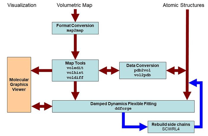
Schematic
diagram of flexing related
routines. Major Situs components (blue) are classified by their
functionality.
The main work flow is indicated by brown arrows. The optional
rebuillding of truncated side chains with the third party SCRWL4
tool is
shown in dark
blue. Visualization
(orange) for the rendering of the data requires a molecular
graphics viewer (we
use
here the
VMD
graphics program,
Chimera and Sculptor also
support Situs
format).
Standard EM
formats are supported
and are converted to cubic lattices in Situs format. This is done with
the map2map
utility. Subsequently,
the data can be inspected and, if necessary, prepared for the fitting
using
a variety of visualization and analysis tools. The ddforge
tool requires one
volume and one PDB structures for the fitting, where all density must
be accounted for. Atomic
coordinates in PDB format can be transformed to low-resolution maps, if
necessary, and vice versa, to allow docking of maps to maps or
structures to structures. The
resulting docked complex can be inspected in the graphics program.
|
| Preparing
the Volume with Map Editing
The ddforge
tool requires
that all density must be accounted for by the fitted PDB file.
Situs provides a number of map tools to adjust the map volume. For an
example how this is done, we refer to the classic Situs tutorial
and Fig.1 of Wriggers et al.
(2011).
|
| Preliminary
Rigid-Body Registration
Before we start
fitting the original
lactoferrin structure to the target map, it is important to roughly
align
the atomic structure and the target map by rigid-body fitting.
An initial alignment
"by eye" can e.g. be done with VMD (move a
loaded molecule by selecting the VMD menu Mouse -> Move
->
Molecule,
then translate it with the mouse and rotate it by pressing the Shift
key; the new coordinates can then be saved by selecting File ->
Save
Coordinates).
Alternatively, an automated
rigid-body fitting
procedure can also be employed. For
an illustrative example, see the actin
fitting example in part II of this tutorial.
|
| Flexible
Refinement with ddforge
This example runs ddforge to fit the PDB
structure "0_lactoferrin_orig.pdb" into the EM map
"0_lactoferrin_target.situs", and uses the residue data from the file
"0_residue_codes_flexible.txt". The remaining parameters used
here are:
1: minimum
displacement between output conformations (Angstrom)
7: map
resolution (Angstrom)
12: density threshold
50: damp/drag ratio
0:
side-chain rebuild flag (0 -> none)
10: force-field
cutoff distance (Angstrom)
1: maximum
displacement per step (Angstrom)
At the shell
prompt enter the following command (see
also run_tutorial.bash):
./ddforge
0_lactoferrin_orig.pdb 0_lactoferrin_target.situs 1 7 12 50 0 10 1 \
-rdfile 0_residue_codes_flexible.txt |
Watch the
program compute a number of iterations until the stopping criterion is
satisfied. The screen output will look like this:
./ddforge
0_lactoferrin_orig.pdb 0_lactoferrin_target.situs 1 7 12 50 0 10 1
-rdfile 0_residue_codes_flexible.txt
ddforge>
ddforge> Atomic structure file: 0_lactoferrin_orig.pdb
ddforge> Density map
file:
0_lactoferrin_target.situs
ddforge> Min. displacement between output confs: 1.000000
ddforge> Map resolution: 7.000000 A
ddforge> Density threshold: 12.000000
ddforge> Damp/drag ratio: 50.000000
ddforge> Side-chain optimization flag: 0
ddforge> Force-field distance cutoff: 10.000000 A
ddforge> Max. displacement per time step: 1.000000 A
ddforge>
ddforge> Reading 0_lactoferrin_orig.pdb
lib_pio> 5332 atoms read from file 0_lactoferrin_orig.pdb.
ddforge>
ddforge> Reading 0_lactoferrin_target.situs
lib_vio> Situs formatted map file 0_lactoferrin_target.situs -
Header information:
lib_vio> Columns, rows, and sections: x=1-103, y=1-96, z=1-82
lib_vio> 3D coordinates of first voxel:
(-33.000000,-33.000000,-64.000000)
lib_vio> Voxel size in Angstrom: 1.000000
lib_vio> Reading density data...
lib_vio> Volumetric data read from file
0_lactoferrin_target.situs
ddforge> Setting density values below 12.000000 to zero.
ddforge>
Optimization of sigma and threshold:
ddforge> iter = 0, sigma =
2.02, threshold_g = 1.42e+01, max_g =
1.14e+02, thr/max(PDB) = 0.124, Gext = 29
ddforge> iter = 1, sigma =
2.42, threshold_g = 3.10e+01, max_g =
1.81e+02, thr/max(PDB) = 0.171, Gext = 35
ddforge> iter = 2, sigma =
2.06, threshold_g = 1.55e+01, max_g =
1.20e+02, thr/max(PDB) = 0.129, Gext = 29
ddforge> iter = 3, sigma =
2.05, threshold_g = 1.51e+01, max_g =
1.18e+02, thr/max(PDB) = 0.128, Gext = 29
ddforge> Number of atoms: 5332
ddforge> Number of pseudo-atoms: 3282
ddforge> Number of residues: 691
ddforge> Read residue-data file '0_residue_codes_flexible.txt'
ddforge> Number of free variables: 1888
ddforge> Number of chains: 1
ddforge> Conf#
Step#
Time
Speed
Disp.
Dist_cut Overlap
Cos Compute time (sec)
ddforge>
0
0 0.000e+00
1.153e-04 5.000e-01
6.543e+01 78.54
0.00000
1.028e+01
ddforge>
1 4.338e+03
8.880e-05 5.000e-01
6.543e+01 78.52
0.00000
1.983e+01
ddforge>
1
2 9.969e+03
6.337e-05 5.178e-01
6.543e+01 78.04
0.99497
2.933e+01
ddforge>
3 1.814e+04
3.954e-05 5.045e-01
5.150e+01 77.30
0.99455
3.917e+01
ddforge>
2
4 3.090e+04
1.650e-05 3.400e-01
3.357e+01 76.57
0.99040
4.861e+01
ddforge>
5 5.150e+04
2.554e-05 3.635e-01
1.679e+01 76.02
0.18558
5.830e+01
ddforge>
6 6.573e+04
9.684e-05 3.922e-01
9.188e+00 77.09
0.92269
6.780e+01
ddforge>
3
7 6.978e+04
9.483e-05 3.624e-01
8.570e+00 78.53
0.98451
7.714e+01
ddforge>
8 7.361e+04
9.614e-05 3.389e-01
7.926e+00 79.80
0.98523
8.662e+01
ddforge>
9 7.713e+04
9.862e-05 3.305e-01
7.372e+00 80.86
0.98511
9.602e+01
ddforge>
4 10
8.048e+04 1.002e-04
3.260e-01 6.926e+00
81.82
0.98767
1.056e+02
ddforge>
11 8.373e+04
1.006e-04 3.131e-01
6.650e+00 82.68
0.98744
1.155e+02
ddforge>
12 8.685e+04
9.459e-05 3.376e-01
6.650e+00 83.47
0.99249
1.251e+02
ddforge>
13 9.041e+04
9.159e-05 3.186e-01
6.650e+00 84.34
0.99389
1.345e+02
ddforge>
5 14
9.389e+04 8.860e-05
2.352e-01 6.650e+00
85.04
0.99161
1.441e+02
ddforge>
15 9.655e+04
8.319e-05 2.082e-01
6.650e+00 85.58
0.99406
1.542e+02
ddforge>
16 9.905e+04
8.123e-05 1.669e-01
6.650e+00 85.96
0.99633
1.639e+02
ddforge>
17 1.011e+05
7.806e-05 1.887e-01
6.650e+00 86.33
0.99706
1.739e+02
ddforge>
18 1.035e+05
7.820e-05 2.116e-01
6.650e+00 86.69
0.99220
1.840e+02
ddforge>
6 19
1.062e+05 8.350e-05
1.949e-01 6.650e+00
86.79
0.96132
1.938e+02
ddforge>
20 1.086e+05
8.142e-05 1.465e-01
6.650e+00 87.04
0.99321
2.039e+02
ddforge>
21 1.104e+05
7.949e-05 1.301e-01
6.650e+00 87.31
0.99604
2.136e+02
ddforge>
22 1.120e+05
7.504e-05 1.561e-01
6.650e+00 87.58
0.99720
2.233e+02
ddforge>
23 1.141e+05
7.323e-05 1.682e-01
6.650e+00 87.83
0.99721
2.327e+02
ddforge>
24 1.164e+05
7.032e-05 2.019e-01
6.650e+00 88.13
0.99642
2.423e+02
ddforge>
25 1.192e+05
6.535e-05 2.095e-01
6.650e+00 88.46
0.99518
2.518e+02
ddforge>
7 26
1.225e+05 6.240e-05
2.302e-01 6.650e+00
88.78
0.99470
2.614e+02
ddforge>
27 1.261e+05
5.973e-05 2.344e-01
6.650e+00 89.09
0.99569
2.713e+02
ddforge>
28 1.301e+05
5.748e-05 2.395e-01
6.650e+00 89.41
0.99602
2.807e+02
ddforge>
29 1.342e+05
5.092e-05 2.285e-01
6.650e+00 89.77
0.99314
2.901e+02
ddforge>
30 1.387e+05
4.595e-05 2.002e-01
6.650e+00 90.18
0.98007
2.995e+02
ddforge>
8 31
1.431e+05 4.240e-05
1.876e-01 6.650e+00
90.50
0.99542
3.090e+02
ddforge>
32 1.475e+05
3.862e-05 1.771e-01
6.650e+00 90.78
0.99702
3.190e+02
ddforge>
33 1.521e+05
3.563e-05 1.734e-01
6.650e+00 91.03
0.99561
3.285e+02
ddforge>
34 1.570e+05
3.163e-05 1.694e-01
6.650e+00 91.31
0.99563
3.381e+02
ddforge>
35 1.623e+05
2.706e-05 1.625e-01
6.650e+00 91.57
0.99145
3.476e+02
ddforge>
36 1.683e+05
2.366e-05 1.627e-01
6.650e+00 91.81
0.98367
3.571e+02
ddforge>
9 37
1.752e+05 1.923e-05
1.637e-01 6.650e+00
92.08
0.97900
3.667e+02
ddforge>
38 1.837e+05
1.676e-05 1.851e-01
6.650e+00 92.37
0.91134
3.766e+02
ddforge>
39 1.947e+05
1.461e-05 1.400e-01
6.650e+00 92.63
0.47895
3.861e+02
ddforge>
40 2.043e+05
1.762e-05 1.503e-01
6.650e+00 92.87
-0.04687
3.955e+02
ddforge>
41 2.129e+05
1.473e-05 6.346e-02
6.650e+00 92.99
-0.36297
4.054e+02
ddforge>
42 2.172e+05
9.249e-06 6.413e-02
6.650e+00 93.15
0.60304
4.155e+02
ddforge>
43 2.241e+05
7.082e-06 7.695e-02
6.650e+00 93.27
0.80377
4.258e+02
ddforge>
44 2.350e+05
6.980e-06 7.109e-02
6.650e+00 93.48
0.71865
4.359e+02
ddforge>
45 2.452e+05
7.484e-06 4.648e-02
6.650e+00 93.66
0.51553
4.455e+02
ddforge>
46 2.514e+05
6.583e-06 5.578e-02
6.650e+00 93.73
0.40252
4.551e+02
ddforge>
10 47
2.598e+05 1.375e-05
6.693e-02 6.650e+00
93.77
0.59082
4.646e+02
ddforge>
48 2.647e+05
6.881e-06 5.812e-02
6.650e+00 93.89
0.84670
4.744e+02
ddforge>
49 2.732e+05
4.894e-06 5.951e-02
6.650e+00 93.99
0.42948
4.839e+02
ddforge>
50 2.853e+05
5.888e-06 7.142e-02
6.650e+00 94.12
0.38010
4.934e+02
ddforge>
51 2.974e+05
1.248e-05 8.570e-02
6.650e+00 94.18
0.19590
5.029e+02
ddforge>
52 3.043e+05
8.516e-06 5.487e-02
6.650e+00 94.28
0.54021
5.125e+02
ddforge>
53 3.108e+05
5.036e-06 2.536e-02
6.650e+00 94.35
0.10986
5.220e+02
ddforge>
54 3.158e+05
5.468e-06 3.044e-02
6.650e+00 94.37
0.31836
5.315e+02
ddforge>
55 3.214e+05
3.696e-06 3.296e-02
6.650e+00 94.43
0.55588
5.410e+02
ddforge>
56 3.303e+05
5.558e-06 3.955e-02
6.650e+00 94.47
0.39599
5.506e+02
ddforge>
57 3.374e+05
4.650e-06 3.239e-02
6.650e+00 94.51
-0.02584
5.601e+02
ddforge>
58 3.444e+05
5.185e-06 2.525e-02
6.650e+00 94.56
-0.34213
5.698e+02
ddforge>
59 3.492e+05
3.635e-06 1.499e-02
6.650e+00 94.60
-0.25787
5.797e+02
ddforge>
60 3.533e+05
3.001e-06 1.653e-02
6.650e+00 94.64
0.30421
5.895e+02
ddforge>
61 3.589e+05
2.683e-06 1.983e-02
6.650e+00 94.66
0.46938
5.992e+02
ddforge>
62 3.662e+05
4.374e-06 2.380e-02
6.650e+00 94.70
0.21611
6.088e+02
ddforge>
63 3.717e+05
2.999e-06 2.443e-02
6.650e+00 94.74
0.48411
6.186e+02
ddforge>
64 3.798e+05
4.804e-06 2.931e-02
6.650e+00 94.79
0.12163
6.283e+02
ddforge>
65 3.859e+05
4.121e-06 2.018e-02
6.650e+00 94.81
-0.28679
6.379e+02
ddforge>
66 3.908e+05
4.084e-06 1.948e-02
6.650e+00 94.86
-0.02655
6.479e+02
ddforge>
67 3.956e+05
2.573e-06 1.360e-02
6.650e+00 94.87
0.15455
6.577e+02
ddforge>
68 4.009e+05
3.510e-06 1.632e-02
6.650e+00 94.89
0.13058
6.675e+02
ddforge>
69 4.055e+05
2.871e-06 1.422e-02
6.650e+00 94.93
0.07488
6.774e+02
ddforge>
70 4.105e+05
3.778e-06 1.707e-02
6.650e+00 94.95
0.05679
6.870e+02
ddforge>
71 4.150e+05
2.521e-06 1.266e-02
6.650e+00 94.98
0.15003
6.973e+02
ddforge>
72 4.200e+05
3.776e-06 1.519e-02
6.650e+00 95.02
0.18649
7.077e+02
ddforge>
73 4.241e+05
2.286e-06 1.168e-02
6.650e+00 95.03
0.35089
7.185e+02
ddforge>
74 4.292e+05
3.022e-06 1.401e-02
6.650e+00 95.05
0.22285
7.290e+02
ddforge>
75 4.338e+05
2.827e-06 1.347e-02
6.650e+00 95.07
0.02903
7.395e+02
ddforge>
76 4.386e+05
3.150e-06 1.616e-02
6.650e+00 95.10
0.06866
7.501e+02
ddforge>
77 4.437e+05
2.682e-06 1.260e-02
6.650e+00 95.11
-0.10886
7.610e+02
ddforge>
78 4.484e+05
2.519e-06 1.134e-02
6.650e+00 95.14
-0.04633
7.718e+02
ddforge>
79 4.529e+05
2.075e-06 1.157e-02
6.650e+00 95.15
0.23405
7.826e+02
ddforge>
80 4.585e+05
2.284e-06 1.389e-02
6.650e+00 95.18
0.10497
7.930e+02
ddforge>
81 4.646e+05
2.508e-06 1.289e-02
6.650e+00 95.19
-0.16646
8.026e+02
ddforge>
82 4.697e+05
2.365e-06 1.084e-02
6.650e+00 95.22
-0.12919
8.122e+02
ddforge>
83 4.743e+05
2.028e-06 1.110e-02
6.650e+00 95.24
0.18948
8.218e+02
ddforge>
84 4.797e+05
2.295e-06 1.291e-02
6.650e+00 95.27
0.02375
8.315e+02
ddforge>
85 4.854e+05
2.484e-06 1.125e-02
6.650e+00 95.29
-0.22301
8.412e+02
ddforge>
11 86
4.899e+05 1.819e-06
8.203e-03 6.650e+00
95.31
-0.00596
8.511e+02
ddforge>
87 4.944e+05
1.858e-06 9.844e-03
6.650e+00 95.33
0.25490
8.610e+02
ddforge>
88 4.997e+05
1.979e-06 1.181e-02
6.650e+00 95.35
0.16621
8.707e+02
ddforge>
89 5.057e+05
2.080e-06 1.094e-02
6.650e+00 95.37
-0.08498
8.802e+02
ddforge>
90 5.109e+05
2.389e-06 1.121e-02
6.650e+00 95.40
-0.10486
8.899e+02
ddforge>
91 5.156e+05
2.306e-06 9.336e-03
6.650e+00 95.41
-0.16474
8.999e+02
ddforge>
92 5.197e+05
2.091e-06 7.102e-03
6.650e+00 95.43
-0.21196
9.101e+02
ddforge>
93 5.231e+05
1.660e-06 7.507e-03
6.650e+00 95.46
0.31350
9.206e+02
ddforge>
94 5.276e+05
1.615e-06 9.008e-03
6.650e+00 95.46
0.37858
9.315e+02
ddforge>
95 5.332e+05
2.070e-06 1.081e-02
6.650e+00 95.48
0.08701
9.421e+02
ddforge>
96 5.384e+05
1.914e-06 9.234e-03
6.650e+00 95.49
-0.08896
9.529e+02
ddforge>
12 96
5.384e+05 1.914e-06
9.234e-03 6.650e+00
95.49
-0.08896
9.529e+02
ddforge>
ddforge> Safe ending time step = 48
ddforge>
ddforge> All done. Program exiting normally.
|
When a line above indicates a conformation # in the first column, a PDB
file is written to disk containing that conformation of the atomic
model, named as the concatenation of the original PDB file name and
"deform.x", where "x" is the conformation number.
The program will end the trajectory according to a stopping criterion
based on the overlap evolution. At the end of the screen output, it
will notify the time step when it is safe to stop the trajectory before
getting into the overfitting regime. It will look like this:
ddforge>
12 96
5.384e+05 1.914e-06
9.234e-03 6.650e+00
95.49
-0.08896
9.529e+02
ddforge>
ddforge> Safe ending time step = 48
ddforge>
ddforge> All done. Program exiting normally.
The safe ending time step will be quite earlier than the current time
step, because sufficient time is needed to assess accurately the start
of the saturation region of the overlap, on which the stopping
criterion is based. Then, the conformation that was written to disk
just before or after the safe ending time step should be taken as the
solution. In the above case, the solution would be the file
0_lactoferrin_orig.deform.10.pdb.
Important preparation for the
next tutorial steps: To prevent overwriting the flexed
files in the subsequent runs below, create a
directory "1_flexible", and move the "deform.x" files into it.
See the run_tutorial.bash file for the respective UNIX commands for
doing this.
|
Using
Residue Constraints
As
specified in the ddforge
user guide and shown
above, one can specify a residue data file that fine-tunes the
refinement of specific amino acid residues. In fact, we could have
omitted this file in the above run as the default program
behavior is
full flexibility. However, the two additional input
files 0_residue_codes_rigid.txt and 0_residue_codes-H+S_rigid-rest_flexible.txt can be used to
demonstrate the effect of full and partial rigidity on the fitted
structure. To explore this, run the above code with these two
alternative residue data files instead. After each run, save
the "deform.x" files to two
new directories "1_rigid" and "1_H+S_rigid-rest_flexible",
respectively. You
should notice that in the fully rigid case the overlap hardly changes
and the program terminates without being able to find a proper stopping
criterion. The partially flexible case (where helices and bends are
rigid and everything else is treated flexible) converges similar to the
above
full flexibility after 47 steps or the 10th conformation.
Secondary structure can be assigned with tools like DSSP. Setting
up residue data files for large PDBs might become labor intensive. You
can use the above templates as a start for other applications.
Alternatively, we
recommend to write a script to generate a template for further editing.
Here we show such a script written in Mathematica, but a user can
probably
translate this to a preferred scripting language without much
difficulty:
|
AllChains
= {{"A", 1, 691}};
ResidueData
= {"CODE CH.ORI.
RES.ORI."};
For[ch =
1, ch <= Length[AllChains], ch++,
chainID = AllChains[[ch, 1]];
res1 = AllChains[[ch, 2]];
g = (Length[AllChains[[ch]]] - 1)/2;
For[s = 1, s <= g, s++,
i1 = AllChains[[ch, 2*s]];
i2 = AllChains[[ch, 2*s + 1]];
For[i = i1, i <= i2, i++,
record = " 31
" <> chainID
<> ToString[PaddedForm[i, 10,
NumberSigns -> {"", ""}]];
AppendTo[ResidueData, record];
]
]
];
Export["residue_data_file.txt",
ResidueData,
"Table"];
|
The
first line specifies the chains and number of residues in the PDB. The
one above is for a particular example of a PDB with a single chain
called A
which has 691 residues. If you had, say, 2 chains, A and B, and chain B
has 200 residues, you would
write
instead: AllChains
= {{"A", 1, 691},
{"B", 10,
200}};
|
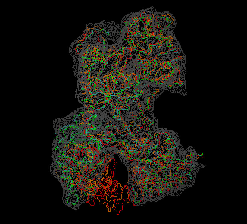
Visualization
We now inspect the above
results with VMD. The following
sequence of commands
in the VMD text console (cf. VMD
user guide) will load the original (red) and flexed
structures (green: flexible; orange: rigid; cyan: partially flexible)
and render them in colored tube representation. The script also renders
the target
density
map in gray.
mol load
pdb 0_lactoferrin_orig.pdb
mol load
pdb 1_flexible/0_lactoferrin_orig.deform.10.pdb
mol load
pdb 1_rigid/0_lactoferrin_orig.deform.4.pdb
mol load
pdb 1_H+S_rigid-rest_flexible/0_lactoferrin_orig.deform.10.pdb
mol load
situs 0_lactoferrin_target.situs
mol top 0
rotate
stop
display
resetview
display
projection orthographic
mol
modstyle
0 0 Lines 2.0
mol modselect 0 0 {name C N CA}
mol
modstyle
0 1 Lines 2.0
mol modselect 0 1 {name C N CA}
mol
modstyle
0 2 Lines 2.0
mol modselect 0 2 {name C N CA}
mol
modstyle
0 3 Lines 2.0
mol modselect 0 3 {name C N CA}
mol
modstyle
0 4 Isosurface 50 0 0 1 2 1
mol
modcolor 0 0 ColorID 1
mol
modcolor 0 1 ColorID 7
mol
modcolor 0 2 ColorID 3
mol
modcolor 0 3 ColorID 10
mol
modcolor 0 4 ColorID 2
|
Don't forget to hit "enter"
after the last line! The result
should look very similar to this image:
(Click
image to
enlarge)
|
| Part
II: Feature-Based Flexible Fitting
If you have low-resolution
(worse than 10A) maps without interior detail, you may be
interested in the original feature-based flexible fitting approach we
initially developed with Joachim Frank and Seth Darst in the early
2000s. Part II of the tutorial shows how to assign simulated features
to the data which can then be used for flexible registration.
Moreover, to improve the
stereochemical quality, it is possible to constrain the
distances between the features to reduce the effect of noise and
other experimental
limitations. This "skeleton" based
approach, as
described on the Vector Quantization
page, is related to 3D
motion capture
technology
used in the entertainment industry and in biomechanics. The
low-resolution applications are demonstrated in the Flexible
Docking Tutorial, Part II.
|
| Return
to the front page . |
|