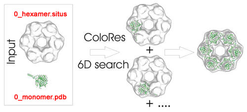
Running colores
For this
particular docking case
it will be sufficient to perform a reduced angular search (sampled at
20°->
option -deg 20) to restore the original atomic structure that we used
to
generate the 15Å simulated EM map (target resolution 15Å
->
option -res 15). After the exhaustive search is done, the best 6
on-lattice
maxima (option -explor 6) will be refined (off-lattice) using
Powell optimization. Here is the command that runs this search:
| ./colores 0_hexamer.situs
0_monomer.pdb -res
15.0
-deg 20 -explor 6 |
When starting
the program (by default as a single processor run), it
will first display the user assigned and default assigned
options. Here you can check if all the input options that
you requested were understood, and if you agree with the default
assignment
of the orther options (the user assigned options are marked in blue).
For
example, at 15Å resolution the program uses by default
the Laplacian filter that enhances
the fitting contrast, and assigns a density threshold of 0.0, i.e. only
positive values will be considered:
|
colores>
Options read:
colores> Target
resolution 15.000 <== -res 15
colores>
Resolution anisotropy 1.000
colores>
Low-resolution map cutoff 0.000
colores>
Laplacian filtered correlation
colores> FFT
grid size expansion factor 0.200 (thickness of additional zero layer as
fraction of map dimensions)
colores> Euler
angles generation using Proportional method
colores>
Angular sampling accuracy 20.000 <== -deg 20
colores> Euler
angle range: [0.000:360.000] [0.000:180.000] [0.000:360.000]
colores>
Sculptor mode OFF
colores> Number
of best fits explored 6 <== -explor 6
colores>
Original peak search by sort and filter
colores> Powell
maximization ON
colores> Powell
tolerance 1.00E-06 Max iterations 25
colores> Powell
trans & rot initial step sizes set to default values
colores> Powell
correlation algorithm determined automatically
colores> Peak
sharpness estimation ON
colores> Number
of SMP processors requested: 1
|
Then the input
files will be read.
You can check if the map parameters, as well as the size of the atomic
structure, are as expected:
colores> Processing low-resolution map.
lib_vio> Situs formatted map file 0_hexamer.situs - Header information:
lib_vio> Columns, rows, and sections: x=1-43, y=1-41, z=1-29
lib_vio> 3D coordinates of first voxel: (-84.000000,-80.000000,-68.000000)
lib_vio> Voxel size in Angstrom: 4.000000
lib_vio> Reading density data...
lib_vio> Volumetric data read from file 0_hexamer.situs
lib_vwk> Setting density values below 0.000000 to zero.
lib_vwk> Remaining occupied volume: 51127 voxels.
lib_vwk> Map size changed from 43 x 41 x 29 to 37 x 35 x 23.
lib_vwk> New map origin (coord of first voxel): (-72.000,-68.000,-56.000)
lib_vwk> Map density info: max 5.881478, min 0.000000, ave 0.709373, sig 1.280587.
_____________________________________________________________________________
colores> Processing atomic structure.
lib_pio> 303 atoms read.
colores> Geometric center: -12.369 -36.951 -9.252, radius: 40.526 Angstrom
|
Next, the
Gaussian filter that
is used for lowering the resolution of the atomic structure, and the
Laplacian
filter that is used to add the contour information to the fitting
criterion,
are generated:
lib_vwk>
Generating Gaussian kernel with 7^3 = 343 voxels.
lib_vwk> Generating Gaussian kernel with 11^3 = 1331 voxels.
lib_vwk> Generating Laplacian kernel with 3^3 = 27 voxels.
lib_vwk> Generating kernel with 9^3 = 729 voxels.
lib_vwk> Map size expanded from 37 x 35 x 23 to 61 x 57 x 41 by
zero-padding.
lib_vwk> New map origin (coord of first voxel):
(-120.000,-112.000,-92.000)
colores> Identifying inside or buried voxels and creating flipped
mask...
colores> Found 11957 inside or buried voxels (out of a total of
142557).
colores> Identifying inside or buried voxels...
colores> Found 11957 inside or buried voxels (out of a total of
142557).
colores> Memory allocation for FFT.
colores> FFT planning...
|
As a test, the
correlation is
calculated with the probe structure centered in target density
map. In this case, since the low resolution map has a "hole" in the
center,
the Laplacian correlation yields negative values:
|
colores> Testing the maps and correlations.
colores> Projecting probe structure to lattice...
colores> Low-pass-filtering probe map...
colores> Target and probe maps:
lib_vwk> Map density info: max 5.881478, min 0.000000, ave 0.148212, sig 0.675602.
lib_vwk> Map density info: max 5.614532, min 0.000000, ave 0.025529, sig 0.279312.
colores> Projecting probe structure to lattice...
colores> Applying filters to target and probe maps...
lib_vwk> Relaxing 5 voxel thick shell about thresholded density...
colores> Normalizing target and probe maps...
colores> Target and probe maps:
lib_vwk> Map density info: max 9.253166, min -12.816330, ave -0.000063, sig 0.560102.
lib_vwk> Map density info: max 16.796933, min -30.926755, ave -0.004420, sig 0.472828.
colores> Writing target and probe maps for inspection or debugging...
lib_vio> Writing density data...
lib_vio> Volumetric data written to file col_hi_fil.sit
lib_vio> File col_hi_fil.sit - Header information:
lib_vio> Columns, rows, and sections: x=1-61, y=1-57, z=1-41
lib_vio> 3D coordinates of first voxel: (-120.000000,-112.000000,-92.000000)
lib_vio> Voxel size in Angstrom: 4.000000
lib_vio> Writing density data...
lib_vio> Volumetric data written to file col_lo_fil.sit
lib_vio> File col_lo_fil.sit - Header information:
lib_vio> Columns, rows, and sections: x=1-61, y=1-57, z=1-41
lib_vio> 3D coordinates of first voxel: (-120.000000,-112.000000,-92.000000)
lib_vio> Voxel size in Angstrom: 4.000000
colores> Computing correlation between maps in direct space...
colores> Correlation with structure centered in density map: -4.2820480E-02
colores> Computing correlation in Fourier space...
colores> FFT correlation with structure centered in density map: -4.2820480E-02
|
Now the uniform
distribution of
the Euler angles that covers the rotational search space is computed.
The
triplets of Euler angles are saved in the file col_eulers.dat. This
file
can be edited or can be used again at other times when you perform a
search
with idenical sampling:
colores>
Getting Euler angles.
lib_eul> Proportional Euler angles distribution, total number 1908
(delta = 20.000000 deg.)
colores> Total number of orientations sampled: 1908
colores> Euler angles saved in file col_eulers.dat.
|
Here follows the
system-dependent
time estimate for the 6D on-lattice search:
colores> Time
of one FFT calculation: 23.093000 ms
colores> Average time spent on each rotation: 47.894200 ms
colores> Estimated time for full 6D (on-lattice) search: 0 h 1 m 31 s
colores> Off-lattice Powell optimization will take significant extra
time.
|
Then the 6D
on-lattice search
is performed. During this search a progressive information about the
best
translational fit for each orientation is written to the file
col_rotate.log. A progress bar keeps you informed:
colores>
Starting 6D on-lattice search with 3D FFT scan of Euler angles.
colores> Searching using 1 processors
colores>
|##################################################|
1908/1908 | 100% done
colores> Actual time spent on 6D on-lattice search: 0 h 1 m 33 s
|
Next follows a peak search
of the maximal correlation values, after which the program enters the
Powell
off-lattice optimization of the selected (-explor) 6 highest scoring
maxima:
colores> Translation function peak detection.
colores> Peak filter contrast: maximum 0.924312, sigma 0.064743
colores> Contrast threshold: 0.129486, candidate peaks: 185
colores> Found 72 non-redundant peaks.
_____________________________________________________________________________
colores> Off-lattice search (Powell's optimization method).
colores> Determining most efficient correlation algorithm based on convergence and time...
colores> Original algorithm: Correlation = -0.01498504 Time = 1.498000 ms
colores> Masked algorithm: Correlation = -0.01506857 Time = 1.376500 ms
colores> One-step algorithm: Correlation = -0.01498504 Time = 1.105000 ms
colores> Using one-step correlation function.
colores> Shown are: offset (in A) from reference center (2.000,2.000,-10.000),
colores> Euler angles (in degrees), and correlation value.
colores>
colores> Performing optimizations...
colores>
colores> Powell optimization for score maximum no. 1.
colores> X
Y
Z Psi
Theta Phi Correlation
colores> 24.000 -32.000 0.000
0.000 0.000 300.000 3.8181654E-01 Initial
colores> 23.718 -31.115 0.621 -0.795 0.132 300.007 3.9282045E-01 1
colores> 23.888 -31.124 0.635 -0.814 0.160 300.008 3.9303528E-01 2
colores> 23.887 -31.124 0.633 -0.814 0.160 300.008 3.9303573E-01 3
colores> 23.887 -31.124 0.633 -0.814 0.160 300.008 3.9303573E-01 4
colores> 23.887 -31.124 0.633 359.186 0.160 300.008 3.9303573E-01 Final
colores>
colores> Powell optimization for score maximum no. 2.
colores> X
Y
Z Psi
Theta Phi Correlation
colores> -28.000 28.000 0.000
0.000 0.000 120.000 3.8181517E-01 Initial
colores> -27.718 27.115 0.621 -0.795 -0.132 120.007 3.9281792E-01 1
colores> -27.888 27.124 0.635 -0.814 -0.160 120.008 3.9303254E-01 2
colores> -27.887 27.124 0.633 -0.814 -0.160 120.008 3.9303300E-01 3
colores> -27.887 27.124 0.633 -0.814 -0.161 120.008 3.9303301E-01 4
colores> -27.887 27.124 0.633 179.186 0.161 300.008 3.9303301E-01 Final
colores>
colores> Powell optimization for score maximum no. 3.
colores> X
Y
Z Psi
Theta Phi Correlation
colores> -40.000 -8.000 0.000
0.000 0.000 60.000 3.6045063E-01
Initial
colores> -40.280 -9.766 0.644 -0.345 -0.085 60.000 3.8385660E-01 1
colores> -40.330 -9.824 0.643 -0.282 -0.052 60.000 3.8393576E-01 2
colores> -40.338 -9.814 0.644 -0.253 -0.047 60.000 3.8394305E-01 3
colores> -40.366 -9.796 0.647 -0.152 -0.031 60.000 3.8396217E-01 4
colores> -40.367 -9.795 0.647 -0.149 -0.031 60.000 3.8396229E-01 5
colores> -40.367 -9.795 0.647 179.851 0.031 240.000 3.8396229E-01 Final
colores>
colores> Powell optimization for score maximum no. 4.
colores> X
Y
Z Psi
Theta Phi Correlation
colores> 36.000 4.000
0.000 0.000 0.000 240.000
3.6044767E-01 Initial
colores> 36.280 5.766 0.644
-0.345 0.085 240.000 3.8385590E-01 1
colores> 36.330 5.824 0.643
-0.282 0.052 240.000 3.8393511E-01 2
colores> 36.338 5.814 0.644
-0.254 0.047 240.000 3.8394234E-01 3
colores> 36.367 5.796 0.647
-0.151 0.031 240.000 3.8396147E-01 4
colores> 36.367 5.795 0.647
-0.149 0.031 240.000 3.8396158E-01 5
colores> 36.367 5.795 0.647
359.851 0.031 240.000 3.8396158E-01 Final
colores>
colores> Powell optimization for score maximum no. 5.
colores> X
Y
Z Psi
Theta Phi Correlation
colores> -16.000 -40.000 0.000
0.000 0.000 0.000
3.5694334E-01 Initial
colores> -14.184 -38.973 0.621 -0.535 -0.365 -0.088 3.9651018E-01 1
colores> -14.301 -39.025 0.653 -0.535 -0.463 -0.141 3.9669580E-01 2
colores> -14.296 -39.054 0.662 -0.535 -0.521 -0.158 3.9670773E-01 3
colores> -14.292 -39.075 0.664 -0.535 -0.531 -0.171 3.9671264E-01 4
colores> -14.292 -39.075 0.666 -0.535 -0.533 -0.171 3.9671285E-01 5
colores> -14.292 -39.075 0.666 179.465 0.533 179.829 3.9671285E-01 Final
colores>
colores> Powell optimization for score maximum no. 6.
colores> X
Y
Z Psi
Theta Phi Correlation
colores> 12.000 36.000 0.000
0.000 0.000 180.000 3.5694033E-01 Initial
colores> 10.184 34.973 0.621 -0.535 0.365 179.912 3.9650980E-01 1
colores> 10.301 35.025 0.653 -0.535 0.463 179.859 3.9669525E-01 2
colores> 10.296 35.053 0.662 -0.535 0.521 179.841 3.9670722E-01 3
colores> 10.292 35.075 0.664 -0.535 0.532 179.829 3.9671214E-01 4
colores> 10.292 35.076 0.666 -0.534 0.533 179.828 3.9671237E-01 5
colores> 10.292 35.076 0.666 359.466 0.533 179.828 3.9671237E-01 Final
colores>
colores> Powell optimization time (6 runs): 10.687460 s
|
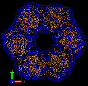
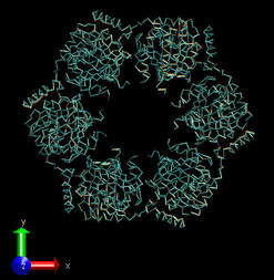
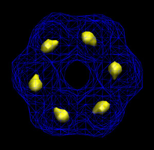
As we
will see later, the six saved fits correspond to the symmetry-related
placement
of the monomer into the hexameric density. The peak sharpness is
estimated for every solution (can be turned off) and the found highest
scoring results are written to PDB files:
colores>
Renormalizing correlation values by highest score.
colores> Writing translation function lattice to Situs file.
lib_vio> Writing density data...
lib_vio> Volumetric data written in Situs format to file col_trans.sit
lib_vio> Situs formatted map file col_trans.sit - Header information:
lib_vio> Columns, rows, and sections: x=1-61, y=1-57, z=1-41
lib_vio> 3D coordinates of first voxel: (-120.000000,-112.000000,-92.000000)
lib_vio> Voxel size in Angstrom: 4.000000
colores> Writing translation function lattice information to log file.
_____________________________________________________________________________
colores> Saving the best results.
colores> Estimating peak sharpness and writing best fit
no. 1 to file col_best_001.pdb.
colores> Estimating peak sharpness and writing best fit
no. 2 to file col_best_002.pdb.
colores> Estimating peak sharpness and writing best fit
no. 3 to file col_best_003.pdb.
colores> Estimating peak sharpness and writing best fit
no. 4 to file col_best_004.pdb.
colores> Estimating peak sharpness and writing best fit
no. 5 to file col_best_005.pdb.
colores> Estimating peak sharpness and writing best fit
no. 6 to file col_best_006.pdb.
|
Finally, in
addion of the output
file coordinates a number of output log files (described in the next
section)
are saved:
colores>
Output files:
col_best*.pdb => Best docking results in PDB format with info in header
col_eulers.dat => colores-readable list of Euler angles
col_rotate.log => Rotation function (unnormalized) log file
col_trans.log => Translation function (norm. by best fit) log file
col_trans.sit => Translation function (norm. by best fit) in Situs format
col_lo_fil.sit => Filtered
target volume in Situs format, just prior to correlation calculation
col_hi_fil.sit => Filtered (and
centered) probe structure in Situs format, just prior to correlation
calculation
col_powell.log => Powell optimization log file
|
|