Classic EM Tutorial, Part I
|
| This tutorial teaches some
basic map editing skills and how to perform a fast
rigid-body
docking of structures to density maps that
were
extracted by difference mapping. The "classic"
tutorial follows the original Situs tutorial of 1999,
therefore it does not cover correlation-based techniques which were
added later in the correlation
and multi-fragment
docking tutorials. Basic functionalities of
many Situs tools are
described in part I below. Part
II describes related but more advanced topics such as density
histogram matching and docking of components to larger maps. The
results can be compared to solutions distributed
with the tutorial
software. More documentation is available in the user
guide, on the methodology
page, and in
the published
articles. |
|
Content:
|
| Download
and Installation
First,
follow these registration
and download steps (each Situs tutorial is separate and must
be downloaded and compiled individually)! Then,
return to this page. The
Situs_3.1_classic_tutorial/bin
directory will contain the executables as well as four input data
files and an executable shell
script:
- 0_ncd.pdb:
Atomic coordinates
of a ncd monomer (as described in Wriggers
et al.,
1999).
- 0_mt.ascii:
ASCII-formatted
density map of the undecorated microtubule (from the Milligan
lab data site).
- 0_nm.ascii:
ASCII-formatted
density map of the ncd monomer decorated microtubule (from the Milligan
lab data site).
- 0_nd.ascii:
ASCII-formatted
density map of the ncd dimer decorated microtubule (from the Milligan
lab data site).
- run_tutorial.bash:
Bash shell script containing all commands of this tutorial.
In the following,
we will
use these four files to dock ncd to the microtubule, following the
steps
described in Wriggers
et al.,
1999. The user
can
compare all generated files to the files in the solutions directory.
|
Data
Flow and Design
The
series
of steps and the programs that are required to dock an
atomic-resolution
structure into a single-molecule, low-resolution EM data are shown
schematically
in the following figure. Detailed program explanations
are
given
in the user guide.
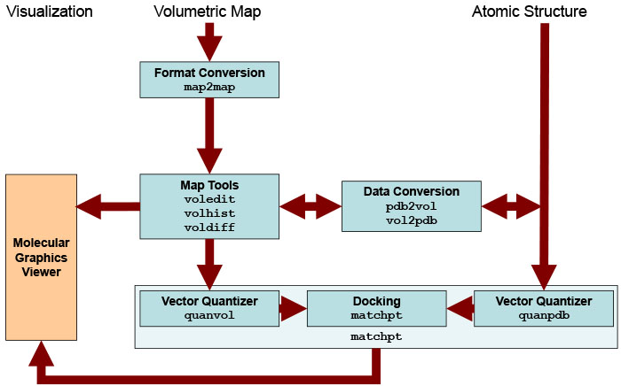
Schematic
diagram of EM related
routines. Major Situs components (blue) are classified by their
functionality.
The main data flow is indicated by brown arrows. The visualization
(orange) for the rendering of the data requires a molecular
graphics viewer (we
use
here the
VMD
graphics program,
Chimera and Sculptor also
support Situs files).
Standard EM
formats are supported
and are converted to cubic lattices in Situs format. This is done with
the map2map
utility. Subsequently, the
data is inspected and, if necessary, prepared for the docking
using a variety of visualization and analysis tools. Situs
docking with matchpt requires one
volume and one PDB structure for the fitting. Atomic
coordinates in PDB format can be transformed to low-resolution maps, if
necessary, and vice versa, to allow docking of maps to maps or
structures to structures. Here we use the classic approach of vector quantization for generating
intermediate coarse grained models of the data. After the
vector quantization, which can be generated by external programs quanvol and quanpdb or which is
automatically generated, the high-resolution structure
is docked to the low-resolution density using matchpt. The resulting
docked complex can be inspected using the external
graphics program.
|
| Converting
the EM Maps
We
convert EM
maps to Situs format
with the map2map
utility. Enter
at
the shell prompt:
| ./map2map
0_mt.ascii 1_mt.situs |
Enter the file
format option 1:
ASCII. Enter the axis order option:
1: X Y Z
(order is
already
correct). Now enter
the number of columns: 89, the
number
of rows: 89, and the number of sections: 61. Enter the grid (lattice)
spacing
in Ångstrom: 6. Finally, enter
the origin of the map: 0 0 0.
Repeat this
procedure similarly
for the other two EM maps to create the files 1_nm.situs and 1_nd.situs
(see run_tutorial.bash).
Here is the map2map
output for file 0_mt.ascii:
./map2map
0_mt.ascii 1_mt.situs
map2map> Input map format not yet recognized.
map2map> Select one of the following input formats (or 0 for
classic menu):
map2map>
map2map> 1:
ASCII (editable text) file, sequential list of map densities**
map2map> 2:
X-PLOR map (ASCII editable text)*
map2map> 3:
Generic 32-bit binary (unknown map or header parameters)
map2map>
map2map> *:
automatic fill of header fields
map2map> **: manual
assignment of header fields
map2map>
map2map> Enter selection: 1
map2map>
map2map> Data order and axis permutation in file 0_mt.ascii.
map2map> Assign columns (C, fastest), rows (R), and sections (S,
slowest) to X, Y, Z:
map2map>
map2map>
C R S =
map2map> ------------------
map2map> 1:
X Y Z (no permutation)
map2map> 2:
X Z Y
map2map> 3:
Y X Z
map2map> 4:
Y Z X
map2map> 5:
Z X Y
map2map> 6:
Z Y X
map2map> Enter selection number [1-6]: 1
map2map> Enter number of columns (X fields): 89
map2map> Enter number of rows (Y fields): 89
map2map> Enter number of sections (Z fields): 61
lib_vio> Reading ASCII data...
lib_vio> Volumetric data read from file 0_mt.ascii
map2map> Enter desired cubic grid (lattice) spacing in Angstrom:
6
map2map>
map2map> Enter X-origin (coord of first voxel) in Angstrom (0 is
recommended, a different value shifts the resulting map accordingly): 0
map2map>
map2map> Enter Y-origin (coord of first voxel) in Angstrom (0 is
recommended, a different value shifts the resulting map accordingly): 0
map2map>
map2map> Enter Z-origin (coord of first voxel) in Angstrom (0 is
recommended, a different value shifts the resulting map accordingly): 0
map2map>
lib_vio> Writing density data...
lib_vio> Volumetric data written in Situs format to file
1_mt.situs
lib_vio> Situs formatted map file 1_mt.situs - Header
information:
lib_vio> Columns, rows, and sections: x=1-89, y=1-89, z=1-61
lib_vio> 3D coordinates of first voxel:
(0.000000,0.000000,0.000000)
lib_vio> Voxel size in Angstrom: 6.000000
map2map>
map2map> All done.
|
Note that the origin of the
coordinate
system is set to the first voxel in the
map.
|
Computing
the Difference Density Maps
We compute
difference density
maps with the voldiff
utility. To
compute
the difference density map of the first, attached ncd monomer, subtract
the microtubule data from the monomer-decorated microtubule data:
| ./voldiff
1_nm.situs 1_mt.situs
2_s1.situs |
Similarly, to
compute the difference
density map of the second, detached monomer, subtract the
monomer-decorated
microtubule data from the dimer-decorated microtubule data:
| ./voldiff
1_nd.situs 1_nm.situs
2_s2.situs |
|
| Inspecting
Data Cross Sections
Now we inspect
the generated Situs
maps with the voledit
utility.
voledit
requires a fixed-width font in the shell window.
First we look at
the dimer-decorated
microtubule. At the shell prompt, enter:
The program
prints the header
information and the minimum and maximum density values of the map. Note
that the default density cutoff for the rendering of voxels is the mean
of the minimum and the maximum density. Enter the desired cross section
type: 1: (x,y)-cross section as function of z-value. The program will
render
the cross section at the half-maximal z position. At the program
prompt,
increase or decrease the z position or enter "0" for changing the
cutoff
value. What happens if you start the program with cross section types
2:
(z,x) or 3: (y,z)? Also inspect the files 1_mt.situs, 1_nm.situs,
2_s1.situs,
and 2_s2.situs (hint: a cutoff value of 12 gives best results for file
2_s2.situs).
Here
is an
example voledit session
for file 1_nd.situs:
./voledit
1_nd.situs
lib_vio> Situs formatted map file 1_nd.situs - Header
information:
lib_vio> Columns, rows, and sections: x=1-89, y=1-89, z=1-61
lib_vio> 3D coordinates of first voxel:
(0.000000,0.000000,0.000000)
lib_vio> Voxel size in Angstrom: 6.000000
lib_vio> Reading density data...
lib_vio> Volumetric data read from file 1_nd.situs
voledit> Min. / max. density values: -31.000000 / 51.000000
voledit> Choose one of the following three options -
voledit> 1:
(x,y)-cross section as
function of z-value
voledit> 2:
(z,x)-cross section as
function of y-value
voledit> 3:
(y,z)-cross section as
function of x-value
voledit> 1
voledit> Box coordinates (1,1,1)=(0.000000,0.000000,0.000000);
(89,89,61)=(534.000000,534.000000,366.000000)
voledit> Cross section at z = 31, display density threshold =
10.000000, display voxel step = 1:
y
^
. . .
. .
. . .
. .
. . .
. .
. . .
. .
. . .- 85
. . .
. .
. . .
. .
. . .
. .
. . .
. .
. . .- 81
. . .
. .
. . .
. .
. . .
. .
. . .
. .
. . .- 77
uuuu
uuu
. . .
. .
. . OOOOOOu
. .OOOO
. . .
. .
. . .
. .
.- 73
OOOOOO ^
. . .
. .
. . uOOOO^
. .
uu. . .
. .
. . .
. .
. .- 69
uuOOOu
uOOOOOu
uOOOO uuuu
. . .
. .OOOOOOOO
^^^OOOOOu . uOOOOOu uuOOOOO .
.
. . .
. .
. .- 65
OOOOOOO
OOOOOu
OOOOOO^OOOOOOOOOu uuuO
. . .
. .
OOOOOOu . OOOOOO
. .
^OOOOOOOOOOOOO .
. .
. . . .- 61
OOOOOOOOOuuuOOOO^
OOOOOOOO uu
. . .
. .
OOOOOOOOOOOOOO^ .
. .
. . ^^^OOOOu uOOOOu
. .
. . .- 57
uOOOOO^OOO^^^OOOOOO^
^OOOOOOOOO^
. . .
uOOOOOO . .OOOOO^
. . .
. .
. . ^OOOOOO^ .
.
. . . .- 53
OOOOOOOOuuOOOOOOO^
^OOO^^
. . .
^OOOOOOOOOOOOOOOO.
. . .
. .
. . .
. uOOOOu
. . . .- 49
^OOOOOOOOOOOOO
uOOOOOOOOOOOOOOu
. . .
. ^OOO^ ^^^^^
. . .
. .
. . .
.uOOOOOOOOOOOOOOOOO
. . .- 45
uuOu
OOOOOO^^ ^^OOOO
. . .
. .
uOOOOOOu. .
. .
. . .
. .uOOO^
. . ^^^ .
. .- 41
uuuuuuuOOOOOOOOO
OOOOOuuuuOOu
. . .
OOOOOOOOOOO^^^Ou.
. . .
. .
. . OOOOOOOOOOOOOO
.
. . .- 37
^^^^^^OO^^
OOOuu
uOOOOOOOOOOOOOOu
. . .
. .
. .uOOOOOOu
. .
. . .
uOOOO^^^^^^OOOOOOOOu. .
. .- 33
uOOOOOOOOuu
OOOOOOu OOOOOOOO
. . .
. .
. uOOO^^^^OOOOOOOu .
. .
uuuOOOOOOOOuuOOOOOOOOOO . .
. .- 29
^^^
OOOOOOOOOOOOuuu OOOOO
^^OOOOOOOOO^^^^O^^
. . .
. .
. . .
OOOOO^^^OOOOOOO OOOOOO
. ^OOOOO^ .
. .
. . .- 25
OOOOO^
OOOO
OOOOOu
. . .
. .
. . .
. .
^^^ . . ^^Ouu .
uOOOOOOu.
. . .
. .- 21
uOOOO OOOOOOO
. . .
. .
. . .
. .
. .
.uOOOOO^. .^^^^
. . .
. .
.- 17
OOOOO^
. . .
. .
. . .
. .
. . .^^^^
.
. . .
. .
. . .- 13
. . .
. .
. . .
. .
. . .
. .
. . .
. .
. . .- 9
. . .
. .
. . .
. .
. . .
. .
. . .
. .
. . .- 5
. . .
. .
. . .
. .
. . .
. .
. . .
. .
. . .- 1
| | |
| |
| | |
| |
| | |
| |
| | |
| |
| | |
1 5 9
13 17 21
25 29 33 37 41
45 49 53
57 61 65 69 73
77 81 85
89 >x
voledit> Increase/decrease z (enter offset value or 0 for more
options):
|
|
Extracting
Regions of Interest
We want to
perform the docking
of the ncd crystal structure to two selected regions of density near
the
microtubule surface. Obviously, the full datasets are too large and
contain
too many individual protein densities. Therefore, we extract first a
small
region of interest near the microtubule surface, using the cropping
tool within voledit
(enter 0 from
within the slice window and 4 on the option menu). An inspection of the
datasets with voledit shows that the 25x25x25 cube with positions
x:57-81,
y:33-57,
z:15-39 is suitable. First, we extract this region from file 1_mt.situs
and save the resulting map to file 3_mt.situs (option 11):
./voledit
1_mt.situs
lib_vio>
Situs formatted map file 1_mt.situs - Header information:
lib_vio> Columns, rows, and sections: x=1-89, y=1-89, z=1-61
lib_vio> 3D coordinates of first voxel:
(0.000000,0.000000,0.000000)
lib_vio> Voxel size in Angstrom: 6.000000
lib_vio> Reading density data...
lib_vio> Volumetric data read from file 1_mt.situs
voledit> Min. / max. density values: -32.000000 / 49.000000
voledit> Choose one of the following three options -
voledit> 1:
(x,y)-cross section as function of z-value
voledit> 2:
(z,x)-cross section as function of y-value
voledit> 3:
(y,z)-cross section as function of x-value
voledit> 1
voledit> Box coordinates (1,1,1)=(0.000000,0.000000,0.000000);
(89,89,61)=(534.000000,534.000000,366.000000)
voledit> Cross-section at z = 31, display density level =
8.500000, display voxel step = 1:
y
^
. . .
. .
. . .
. .
. . .
. .
. . .
. .
. . .- 85
. . .
. .
. . .
. .
. . .
. .
. . .
. .
. . .- 81
. . .
. .
. . .
. .
. . .
. .
. . .
. .
. . .- 77
. . .
. .
. . .
. .
. . .
. .
. . .
. .
. . .- 73
. . .
. .
. . .
. .
uuOu. . .
.
. . .
. .
. . .- 69
OOOOOOu
uuOOu
. . .
. .
. . .
uOOuu. OOOOOOOuuOOOOOOO
. . .
. .
. . . .- 65
OOOOOOu
OOOOOOOOOOOOOOOOOuuuuu
. . .
. .
. . . OOOOOOOO .^^ .
^OOOOOOOOOOOOOOO . .
.
. . . .- 61
u
OOOOOOOOOOO^
^OOOOOOOOO
. . .
. .
. .OOOOOOOO^^ .
. .
. .^^OOOOOOuuu.
. .
. . . .- 57
OOOOOOO
^OOOOOOOOu
. . .
. . .
uuuOOOOOO . .
. .
. . . ^OOOOOOOO
. .
. . . .- 53
OOOOOOOO^^
^OOOO^
. . .
. .
.OOOOOOOO .
. .
. . .
. .^^
. . .
. .
. .- 49
^OOOOOOO
uOOOOOu
. . .
. .
. ^^^O^. .
. .
. . .
.
.OOOOOOOO .
. .
. .- 45
uuOOO
OOOOOOOO
. . .
. .
uOOOOOOu. .
. .
. . .
.
uOOOOO^^. .
. .
. .- 41
OOOOOOOO
OOOOOOu
. . .
. .
.^^^OO^Ouu . .
.
. . .
. OOOOOOO
. . .
. .
.- 37
OOOOuu
uOOOOOOOOO
. . .
. .
. .OOOOOOOOu .
.
. . .
OOOOOOOOOO
. . .
. .
.- 33
^OOOOOOOOOuuuu
uOOOOOOO
. . .
. .
. .^^^^^OOOOOOOOOu.
. .
uuuOOOOOOOOO . .
.
. . . .- 29
OOOOOOOOOOOOOOu
uuOOOOOO^^OOOO
. . .
. .
. . . OOOOOOOOOOOOOOO
^OOOOOOO
. . .
. .
. . . .- 25
^^^ ^OOOOOO^
^OOOOO^
. . .
. .
. . .
. .
^OOO^. . ^^^
. .
. . .
. .
. .- 21
. . .
. .
. . .
. .
. . .
. .
. . .
. .
. . .- 17
. . .
. .
. . .
. .
. . .
. .
. . .
. .
. . .- 13
. . .
. .
. . .
. .
. . .
. .
. . .
. .
. . .- 9
. . .
. .
. . .
. .
. . .
. .
. . .
. .
. . .- 5
. . .
. .
. . .
. .
. . .
. .
. . .
. .
. . .- 1
| | |
| |
| | |
| |
| | |
| |
| | |
| |
| | |
1 5 9
13 17 21
25 29 33 37 41
45 49 53
57 61 65 69 73
77 81 85
89 >x
voledit> Browse slices (sections z=1-61, projection z=0):
pos/neg int for up/down or 0 for more options: 0
voledit> Choose one of the following options:
voledit>
1: Set cross-section z index or select projection
voledit>
2: Set display density level
voledit>
3: Set voxel step for display
voledit>
4: Cropping (cut away margin)
voledit>
5: Zero padding (extra margin)
voledit>
6: Interpolation (change voxel spacing)
voledit>
7: Polygon clippling
voledit>
8: Segmentation (floodfill) of contiguous volume
voledit>
9: Thresholding (set low densities to zero)
voledit> 10:
Binary thresholding (set densities to zero or one)
voledit> 11:
Save current slice
voledit> 12:
Save entire map
voledit> 13:
Quit voledit
voledit> 4
voledit> Voxel range of cropping. Enter new grid values:
voledit> Minimum x value (1-89): 57
voledit> Maximum x value (57-89): 81
voledit> Minimum y value (1-89): 33
voledit> Maximum y value (33-89): 57
voledit> Minimum z value (1-61): 15
voledit> Maximum z value (15-61): 39
lib_vwk> 89 x 89 x 61 map projected to 25 x 25 x 25 lattice.
lib_vwk> New map origin (coord of first voxel):
(336.000,192.000,84.000)
voledit> Box coordinates
(1,1,1)=(336.000000,192.000000,84.000000);
(25,25,25)=(486.000000,342.000000,234.000000)
voledit> Cross-section at z = 13, display density level =
8.000000, display voxel step = 1:
y
^
^OOOOOOOu
. OOOOOOOOOu. .
. .- 21
^^OOOOOOO
. OOOOOO .
. . .- 17
OOOOOOOu
. ^OOOOOOOO
. . .- 13
OOOOOOO^
. .OOOO^ .
. . .- 9
uOOOOu
. OOOOOOO .
. . .- 5
OOOOOOO
uuuu. ^^^^ . .
. .- 1
| | |
| | |
|
1 5 9
13 17 21 25 >x
voledit> Browse slices (sections z=1-25, projection z=0):
pos/neg int for up/down or 0 for more options: 0
voledit> Choose one of the following options:
voledit>
1: Set cross-section z index or select projection
voledit>
2: Set display density level
voledit>
3: Set voxel step for display
voledit>
4: Cropping (cut away margin)
voledit>
5: Zero padding (extra margin)
voledit>
6: Interpolation (change voxel spacing)
voledit>
7: Polygon clippling
voledit>
8: Segmentation (floodfill) of contiguous volume
voledit>
9: Thresholding (set low densities to zero)
voledit> 10:
Binary thresholding (set densities to zero or one)
voledit> 11:
Save current slice
voledit> 12:
Save entire map
voledit> 13:
Quit voledit
voledit> 12
voledit> Enter
filename for the modified map: 3_mt.situs
lib_vio>
Writing density data...
lib_vio> Volumetric data written in Situs format to file
3_mt.situs
lib_vio> Situs formatted map file 3_mt.situs - Header
information:
lib_vio> Columns, rows, and sections: x=1-25, y=1-25, z=1-25
lib_vio> 3D coordinates of first voxel:
(336.000000,192.000000,84.000000)
lib_vio> Voxel size in Angstrom: 6.000000
|
Similarly, (see
the run_tutorial.bash script) we
create the files
3_nd.situs, 3_nm.situs, 3_s1.situs, and 3_s2.situs from the
corresponding
files 1_nd.situs, 1_nm.situs, 2_s1.situs, and 2_s2.situs.
|
Inspecting
the Voxel Histogram
Next, we inspect
the file 3_nm.situs
with the program volhist
to make
sure
the background peak in the voxel histogram is at the origin. When
prompted, enter the number of histogram bins (40):
./volhist
3_nm.situs
lib_vio>
Situs formatted map file 3_nm.situs - Header information:
lib_vio> Columns, rows, and sections: x=1-25, y=1-25, z=1-25
lib_vio> 3D coordinates of first voxel:
(336.000000,192.000000,84.000000)
lib_vio> Voxel size in Angstrom: 6.000000
lib_vio> Reading density data...
lib_vio> Volumetric data read from file 3_nm.situs
lib_vwk> Density information. min: -27.000000 max: 50.000000
ave: 6.590784 sig: 15.990164 norm: 17.295195
lib_vwk> Above zero density information. ave: 17.834073 sig:
13.150531 norm: 22.158309
lib_vwk> Please enter the of number histogram bins: 40
lib_vwk> Printing voxel histogram, 40 histogram bins
lib_vwk> (density value; voxel count; top-down cumulative volume
fraction):
-27.000 | 2
.
. . .
. .
. . .
. .
. . .
. .
. . . |
1.000e+00
-25.026 |=
27
| 9.999e-01
-23.051 |==== 94
. .
. . .
. .
. . .
. .
. . .
. . |
9.981e-01
-21.077 |=======
157
| 9.921e-01
-19.103 |======== 193
. .
. . .
. .
. . .
. .
. . .
. | 9.821e-01
-17.128 |============
287
| 9.697e-01
-15.154 |============== 323 .
.
. . .
. .
. . .
. .
. . . |
9.514e-01
-13.179 |=============
307
| 9.307e-01
-11.205 |============== 319 .
.
. . .
. .
. . .
. .
. . . |
9.110e-01
-9.231 |===============
350
| 8.906e-01
-7.256 |======================== 548
.
. . .
. .
. . .
. .
. | 8.682e-01
-5.282 |================================
717
| 8.332e-01
-3.308
|=====================================================
1185 . . .
.
. | 7.873e-01
-1.333
|======================================================================
1565 | 7.114e-01
0.641
|=======================================================================->
1761 | 6.113e-01
2.615 |===========================================
966
| 4.986e-01
4.590 |===============================
714 .
. .
. . .
. .
. . | 4.367e-01
6.564 |====================
459
| 3.910e-01
8.538 |===============
355 .
. . .
. .
. . .
. .
. . . |
3.617e-01
10.513 |================
358
| 3.389e-01
12.487 |============== 328 .
.
. . .
. .
. . .
. .
. . . |
3.160e-01
14.462 |===============
349
| 2.950e-01
16.436 |============== 325 .
.
. . .
. .
. . .
. .
. . . |
2.727e-01
18.410 |=============
305
| 2.519e-01
20.385 |=============== 342
.
. . .
. .
. . .
. .
. . . |
2.324e-01
22.359 |==============
322
| 2.105e-01
24.333 |============= 300 .
.
. . .
. .
. . .
. .
. . . |
1.899e-01
26.308 |=============
295
| 1.707e-01
28.282 |============== 326 .
.
. . .
. .
. . .
. .
. . . |
1.518e-01
30.256 |===============
353
| 1.309e-01
32.231 |============== 321 .
.
. . .
. .
. . .
. .
. . . |
1.084e-01
34.205 |=============
303
| 8.781e-02
36.179 |============== 317 .
.
. . .
. .
. . .
. .
. . . |
6.842e-02
38.154 |============
278
| 4.813e-02
40.128 |========= 211 .
.
. . .
. .
. . .
. .
. . .
. | 3.034e-02
42.103 |======
137
| 1.683e-02
44.077 |=== 74 . .
.
. . .
. .
. . .
. .
. . .
. . |
8.064e-03
46.051 |=
40
| 3.328e-03
48.026 | 11
. .
. . .
. .
. . .
. .
. . .
. .
. | 7.680e-04
50.000 |
1
| 6.400e-05
lib_vwk> Maximum at density
value 0.641
|
The above inspection
shows that the
background peak is already at the origin, so there is nothing to do
here. However, if necessary volhist
could be run with additional file names as
arguments,
in which case the program would provide options for rescaling or
shifting the densities, or for matching the density histogram of two
maps. The more advanced functionality is described in part
II of this tutorial.
|
Extracting
Single-Molecule Densities
We are now
prepared to extract
single-molecule densities with the floodfill segmentation
utility within voledit (enter 0 from
within the slice
window, then 8 on the option menu).
Inspection of the file 3_s1.situs
with voledit indicates that the voxel at position x=16, y=16,
z=16
is located near the center of the density of an attached monomer that
can be isolated at a threshold level of 20. After applying floodfill we
also use thresholding at this level to eliminate any outside density.
Here is
the voledit session for extracting the first monomer and writing it to
file 4_s1.situs:
./voledit
3_s1.situs
lib_vio> Situs formatted map file 3_s1.situs - Header
information:
lib_vio> Columns, rows, and sections: x=1-25, y=1-25, z=1-25
lib_vio> 3D coordinates of first voxel:
(336.000000,192.000000,84.000000)
lib_vio> Voxel size in Angstrom: 6.000000
lib_vio> Reading density data...
lib_vio> Volumetric data read from file 3_s1.situs
voledit> Min. / max. density values: -19.000000 / 56.000000
voledit> Choose one of the following three options -
voledit> 1:
(x,y)-cross section as function of z-value
voledit> 2:
(z,x)-cross section as function of y-value
voledit> 3:
(y,z)-cross section as function of x-value
voledit> 1
voledit> Box coordinates
(1,1,1)=(336.000000,192.000000,84.000000);
(25,25,25)=(486.000000,342.000000,234.000000)
voledit> Cross-section at z = 13, display density level =
18.500000, display voxel step = 1:
y
^
^OOOO^
. . .
^. . . .-
21
. . .
uOOOOOO . .- 17
^OOOOOO
. . .
.OOOO^ . .- 13
. . .
. . . .-
9
. . .
uuuu. . .- 5
OOOOO
. . . ^^^
. . .- 1
| | |
| | |
|
1 5 9
13 17 21 25 >x
voledit> Browse slices (sections z=1-25, projection z=0):
pos/neg int for up/down or 0 for more options: 0
voledit> Choose one of the following options:
voledit>
1: Set cross-section z index or select projection
voledit>
2: Set display density level
voledit>
3: Set voxel step for display
voledit>
4: Cropping (cut away margin)
voledit>
5: Zero padding (extra margin)
voledit>
6: Interpolation (change voxel spacing)
voledit>
7: Polygon clippling
voledit>
8: Segmentation (floodfill) of contiguous volume
voledit>
9: Thresholding (set low densities to zero)
voledit> 10:
Binary thresholding (set densities to zero or one)
voledit> 11:
Save current slice
voledit> 12:
Save entire map
voledit> 13:
Quit voledit
voledit> 8
voledit> Min. / max. density values: -19.000000 / 56.000000
voledit> Enter desired threshold level for floodfill
segmentation: 20
voledit> Enter floodfill start index x (1-25): 16
voledit> Enter floodfill start index y (1-25): 16
voledit> Enter floodfill start index z (1-25): 16
voledit> 3D coordinates of start grid point (16,16,16):
(426.00,282.00,174.00)
voledit> Shrink map about found volume? Choose one of the
following options:
voledit>
voledit> 1: No
(keep input map size)
voledit> 2:
Yes (shrink map)
2
voledit> Filling contiguous volume...
voledit> Filling contiguous volume...
voledit> Contiguous volume, > 20.000000: 284 voxels
(6.134400e+04 Angstrom^3)
voledit> Extracted volume, > 0.000000: 724 voxels
(1.563840e+05 Angstrom^3)
lib_vwk> 25 x 25 x 25 map projected to 9 x 10 x 14 lattice.
lib_vwk> New map origin (coord of first voxel):
(396.000,252.000,132.000)
voledit> Box coordinates
(1,1,1)=(396.000000,252.000000,132.000000);
(9,10,14)=(450.000000,312.000000,216.000000)
voledit> Cross-section at z = 8, display density level =
27.000000, display voxel step = 1:
y
^
. . .- 9
OOOO
. OOOOO .- 5
OOOO
. . .- 1
| | |
1 5 9
>x
voledit> Browse slices (sections z=1-14, projection z=0):
pos/neg int for up/down or 0 for more options: 0
voledit> Choose one of the following options:
voledit>
1: Set cross-section z index or select projection
voledit>
2: Set display density level
voledit>
3: Set voxel step for display
voledit>
4: Cropping (cut away margin)
voledit>
5: Zero padding (extra margin)
voledit>
6: Interpolation (change voxel spacing)
voledit>
7: Polygon clippling
voledit>
8: Segmentation (floodfill) of contiguous volume
voledit>
9: Thresholding (set low densities to zero)
voledit> 10:
Binary thresholding (set densities to zero or one)
voledit> 11:
Save current slice
voledit> 12:
Save entire map
voledit> 13:
Quit voledit
voledit> 9
voledit> Enter threshold level (densities below this will be set
to zero): 20
lib_vwk> Setting density values below 20.000000 to zero.
lib_vwk> Remaining occupied volume: 284 voxels.
voledit> Box coordinates
(1,1,1)=(396.000000,252.000000,132.000000);
(9,10,14)=(450.000000,312.000000,216.000000)
voledit> Cross-section at z = 8, display density level =
27.000000, display voxel step = 1:
y
^
. . .- 9
OOOO
. OOOOO .- 5
OOOO
. . .- 1
| | |
1 5 9
>x
voledit> Browse slices (sections z=1-14, projection z=0):
pos/neg int for up/down or 0 for more options: 0
voledit> Choose one of the following options:
voledit>
1: Set cross-section z index or select projection
voledit>
2: Set display density level
voledit>
3: Set voxel step for display
voledit>
4: Cropping (cut away margin)
voledit>
5: Zero padding (extra margin)
voledit>
6: Interpolation (change voxel spacing)
voledit>
7: Polygon clippling
voledit>
8: Segmentation (floodfill) of contiguous volume
voledit>
9: Thresholding (set low densities to zero)
voledit> 10:
Binary thresholding (set densities to zero or one)
voledit> 11:
Save current slice
voledit> 12:
Save entire map
voledit> 13:
Quit voledit
voledit> 12
voledit> Enter filename for the modified map: 4_s1.situs
lib_vio> Writing density data...
lib_vio> Volumetric data written to file 4_s1.situs
lib_vio> Situs formatted map file 4_s1.situs - Header
information:
lib_vio> Columns, rows, and sections: x=1-9, y=1-10, z=1-14
lib_vio> 3D coordinates of first voxel:
(396.000000,252.000000,132.000000)
lib_vio> Voxel size in Angstrom: 6.000000
voledit> Box coordinates
(1,1,1)=(396.000000,252.000000,132.000000);
(9,10,14)=(450.000000,312.000000,216.000000)
voledit> Cross-section at z = 8, display density level =
27.000000, display voxel step = 1:
y
^
. . .- 9
OOOO
. OOOOO .- 5
OOOO
. . .- 1
| | |
1 5 9
>x
voledit> Browse slices (sections z=1-14, projection z=0):
pos/neg int for up/down or 0 for more options: 0
voledit> Choose one of the following options:
voledit>
1: Set cross-section z index or select projection
voledit>
2: Set display density level
voledit>
3: Set voxel step for display
voledit>
4: Cropping (cut away margin)
voledit>
5: Zero padding (extra margin)
voledit>
6: Interpolation (change voxel spacing)
voledit>
7: Polygon clippling
voledit>
8: Segmentation (floodfill) of contiguous volume
voledit>
9: Thresholding (set low densities to zero)
voledit> 10:
Binary thresholding (set densities to zero or one)
voledit> 11:
Save current slice
voledit> 12:
Save entire map
voledit> 13:
Quit voledit
voledit> 13
voledit> Bye bye!
|
Now do the same
for the second,
detached monomer (see
the run_tutorial.bash script). Similarly,
one finds that the voxel at position x=19, y=12, z=13 is located near
the
center of the density of the detached monomer in file 3_s2.situs at a
threshold level of 12. The threshold cutoff values
were found
by
trial
and error to prevent "leaking"
of the density into neighboring monomers. Here we also shrink the maps
about the found extracted volumes.
|
| Vector
Quantization and Docking
Now we
can perform the vector
quantization
and fast docking of the attached monomer with the matchpt
utility. At the shell prompt, enter
| ./matchpt
NONE 4_s1.situs NONE 0_ncd.pdb |
using the default parameters of matchpt. NONE are place
holders for so-called codebook
vectors (a coarse-grained model used
for fast point-cloud matching). The usage of NONE instead
of explicit file names specifies that missing codebook
vectors will be calculated in the
fly.
Watch the
program vector quantize
the atomic and low-resolution data for a (default) range of 4-9
codebook vectors. For each number of vectors, a small number of
calculations are repeated with different random number seeds
for
both atomic and low-resolution data. The averaged codebook vectors are
then used for the matching, and their rms variability is displayed.
After
computing
the N (M) vectors for high- (low-) resolution data (M ≈ units * N, where
units is by default set to 1), the subsequent
docking
then determines the six rigid-body degrees of freedom by a
least-squares
fit of matching pairs of vectors. The corresponding vectors
are not known a priori, and a large number of possible combinations are
explored. Good matches are found for select numbers N, M, and the best number of
vectors (here: N, M=7) is chosen by the lowest resulting rms
deviation (RMSD).
The
program returns a list of solutions for (N, M=7), ranked by
their codebook
vector rms deviation. The correlation coefficient is also shown. The
fourth
column in the output below shows the internal permutation of the
vectors that determine the
superposition. Note that the correlation
coefficient
is within a very narrow numeric range, despite the significant
differences
in orientation between these fits, whereas the vector rmsd is more
discriminatory.
To
prevent the resulting files from being over written, we save the two
best solutions to the files 5_s1_1.dock.pdb and 5_s1_2.dock.pdb,
respectively, and delete all other output which is no longer needed.
Here
is the
output of the entire matchpt calculation, including the UNIX shell
commands at the end that save the best two fits and remove all other
output:
./matchpt
NONE 4_s1.situs NONE 0_ncd.pdb
matchpt> File1 == NONE
lib_vio> Situs formatted map file 4_s1.situs - Header
information:
lib_vio> Columns, rows, and sections: x=1-9, y=1-10, z=1-14
lib_vio> 3D coordinates of first voxel:
(396.000000,252.000000,132.000000)
lib_vio> Voxel size in Angstrom: 6.000000
lib_vio> Reading density data...
lib_vio> Volumetric data read from file 4_s1.situs
matchpt> File3 == NONE
matchpt> Loading high-resolution structure PDB file: 0_ncd.pdb
matchpt> No codebook vectors available, will compute a series of
vector
matchpt> sets of different sizes and rank them.
matchpt>
matchpt> Computation and clustering of sets of (high res./low
res.) codebook vectors.
lib_mpt> Variability
of 4 codebook vectors in 8 statistically independent runs:
0.376 A
lib_mpt> Variability of 5 codebook vectors in 8
statistically independent runs: 1.464 A
lib_mpt> Variability of 6 codebook vectors in 8
statistically independent runs: 1.048 A
lib_mpt> Variability of 7 codebook vectors in 8
statistically independent runs: 1.089 A
lib_mpt> Variability of 4 codebook vectors in 8
statistically independent runs: 1.317 A
lib_mpt> Variability of 5 codebook vectors in 8
statistically independent runs: 0.457 A
lib_mpt> Variability of 6 codebook vectors in 8
statistically independent runs: 1.837 A
lib_mpt> Variability of 7 codebook vectors in 8
statistically independent runs: 0.328 A
lib_mpt> Variability of 8 codebook vectors in 8
statistically independent runs: 1.773 A
lib_mpt> Variability of 9 codebook vectors in 8
statistically independent runs: 2.522 A
lib_mpt> Variability of 8 codebook vectors in 8
statistically independent runs: 3.074 A
lib_mpt> Variability of 9 codebook vectors in 8
statistically independent runs: 0.409 A
matchpt>
matchpt> Point cloud matching for (high res./low res.) vectors:
matchpt> 4/4 vectors: No matches found.
matchpt> 6/6 vectors: No matches found.
matchpt> 8/8 vectors: No matches found.
matchpt> 5/5 vectors: 2 matches found with min RMSD 3.744 A,
variabilities 0.457/1.464 A, max CC 0.883
matchpt> 9/9 vectors: 1 match found with RMSD 5.086 A,
variabilities 0.409/2.522 A, CC: 0.857
matchpt> 7/7 vectors: 6 matches found with min RMSD 2.712 A,
variabilities 0.328/1.089 A, max CC 0.897
matchpt>
matchpt> Based on min RMSD, selecting 6 matches from 7/7
vectors. Exploring top 6 RMSD solutions.
matchpt>
matchpt> Solution filename, codebook vector RMSD in Angstrom,
matchpt> cross-correlation coefficient, and permutation
matchpt> (order of low res fitted to high res vectors):
matchpt>
matchpt> mpt_001.pdb - RMSD: 2.712
CC: 0.897 - ( 3, 4, 2, 6, 7, 5, 1)
matchpt> mpt_002.pdb - RMSD: 4.334
CC: 0.852 - ( 4, 7, 2, 1, 3, 6, 5)
matchpt> mpt_003.pdb - RMSD: 5.116
CC: 0.849 - ( 7, 3, 2, 5, 4, 1, 6)
matchpt> mpt_004.pdb - RMSD: 7.964
CC: 0.834 - ( 1, 7, 5, 3, 4, 2, 6)
matchpt> mpt_005.pdb - RMSD: 8.249
CC: 0.754 - ( 5, 3, 6, 4, 7, 2, 1)
matchpt> mpt_006.pdb - RMSD: 9.084
CC: 0.722 - ( 6, 4, 1, 7, 3, 2, 5)
matchpt>
matchpt> All done.
|
Now do the same
for the second,
detached monomer. Is there a unique best fit? What is the lowest rms
deviation
and the gap to the subsequent fits? Extract the best fit to the file
5_s2_1.dock.pdb and the
second best to 5_s2_2.dock.pdb. See also the run_tutorial.bash script
for details on automating these steps.
Note: As described in (Birmanns
& Wriggers, 2007), the fast matching
by codebook vectors can be refined by a post-processing with the
correlation-based tool collage.
We
have explained this refinement step in the separate multi-fragment docking tutorial.
|
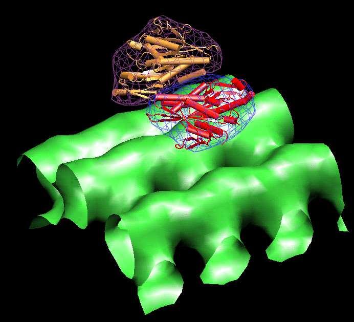
Visualization
This section
uses the graphics
program VMD. Chimera and Sculptor also
support Situs
format.
Note that the
origin of the Situs map coordinate system was
assigned
by map2map.
The following
sequence of commands
in the VMD text console (cf. VMD
user
guide) will load the two docked structures, 5_s1_1.dock.pdb
and
5_s2_1.dock.pdb, and render them in cartoon representation, coded by
color.
The script then instructs VMD to render the density maps 3_mt.situs in green,
4_s1.situs in
blue, and 4_s2.situs in purple:
mol load
pdb 5_s1_1.dock.pdb
mol load
pdb
5_s2_1.dock.pdb
mol load
situs 3_mt.situs
mol load
situs 4_s1.situs
mol load
situs 4_s2.situs
mol top 0
rotate
stop
display
resetview
display
projection orthographic
mol
modstyle
0 0 Cartoon 2.1 11
5
mol
modstyle
0 1 Cartoon 2.1 11
5
mol
modstyle
0 2 Isosurface 20 0 0 0 1 1
mol
modstyle
0 3 Isosurface 20 0 0 1 1 1
mol
modstyle
0 4 Isosurface 12 0 0 1 1 1
mol
modcolor
0 0 ColorID 1
mol
modcolor
0 1 ColorID 3
mol
modcolor
0 2 ColorID 7
mol
modcolor
0 3 ColorID 0
mol
modcolor
0 4 ColorID 11
|
Don't forget to hit "enter"
after the last line!
The
result
should look like this:
(Click
image to
enlarge)
|
| Part
II: Advanced Matching with volhist
and matchpt
The matchpt tool supports the
registration of point clouds even in cases where they are of unequal
size, such as in oligomeric assemblies. Also, as mentioned above, volhist provides
options for rescaling or shifting the densities, or for matching the
density histogram of two maps. The more advanced usage of
these
routines is demonstrated on the above examples in part II
of this
tutorial.
|
| Return
to the front page . |
|