|
SAXS Tutorial
|
| The tutorial
teaches the modeling and visualization
of low resolution bead models
of
protein structures derived from small angle X-ray scattering. The
results
can be compared to solutions distributed with the tutorial software. In
the demonstration below we use two cross-correlation based rigid body
strategies for the docking. However, the user may employ also
other fitting strategies as discussed under Outlook.
Once density maps are created, the rigid-body and flexible docking of
structures
to SAXS bead models is very similar to the approach used for electron
microscopy
maps. More documentation is available in the user
guide, in the methodology
page, and in
the published articles. |
|
Content:
|
Download
and Installation
Then, return to this page.
The
Situs_3.1_saxs_tutorial/bin directory will contain the executables as well as four input data
files and an executable shell
script:
- 0_tnc.pdb:
Atomic coordinates
of troponin C.
- 0_rib.pdb:
Atomic coordinates
of ribonuclease inhibitor.
- 0_tnc_sph.pdb:
Bead model
of troponin C.
- 0_rib_sph.pdb:
Bead model
of ribonuclease inhibitor.
- run_tutorial.bash:
Bash shell script containing all commands of this tutorial.
Note that the bead
model files are
in PDB format, with the bead sphere radius in the occupancy field. In
the
following, we will perform various modeling tasks.
The user can compare all generated files to the files in the
"solutions"
directory.
|
Data
Flow and Design
The
series
of steps and the utilities that are required for the modeling with
single-molecule SAXS bead models are shown
schematically
in the following figure. Bead models are expected to
result
from experimental reconstructions. Simulated bead models for validation
of the modeling strategies can also be created with pdb2sax. Detailed program
explanations are
given
in the user guide.
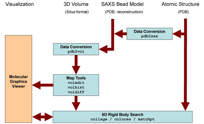
Schematic
diagram of SAXS related
routines. Major Situs components (blue) are classified by their
functionality.
The main data flow is indicated by brown arrows. The visualization
(orange) for the rendering of the bead models requires a molecular
graphics viewer (we
use
here the
VMD
graphics program,
Chimera and Sculptor also
support Situs
format).
Visualization and modeling
of
atomic structures into SAXS bead models
are supported through a conversion into 3D volumes with the pdb2vol kernel convolution tool.
A docking between atomic structures to 3D maps can be achieved with a
number of approaches (see below). The resulting docked complex can be
inspected using a
molecular graphics viewer. The data can be prepared further
for the visualization using a variety of analysis and editing
tools. Kernel convolution facilitates the smoothing of bead surfaces
for
their visualization in the form of density isocontours.
|
Converting
Volumetric Bead Maps
The creation of simulated
bead models
on a hexagonal lattice with pdb2sax
is straightforward and will not be discussed here in further detail. We assume that bead models
are
already available from experimental reconstructions. We first convert SAXS
bead models to
volumetric Situs format with the pdb2vol
kernel convolution utility. Enter at the shell prompt:
| ./pdb2vol
0_rib_sph.pdb
1_rib_sph.situs |
Select no
mass-weighting (enter
1) and no B-factor thresholding (enter 1), then enter the desired voxel
spacing of the output map. Given the
dimensions
of the structure and the bead radius (6 Å), 1Å
appears
to
be a good compromise between bead sampling accuracy and storage
requirement (you may have to adjust this value upwards for other cases
to avoid oversampling of beads and resulting large maps).
Next, enter the kernel width (bead radius): +6 Å. This is the
half-max
radius where the kernel amplitude drops to its half maximal
value.
Next, select the "Hard Sphere" smoothing kernel (enter 5). Turn lattice
correction off (enter 2), and enter the maximum amplitude of the kernel
(enter
1 and keep a note of this).
The program
projects the atomic
structure to the lattice, computes the hard sphere kernel, and carries
out the real-space convolution, writing the resulting map to the file
1_rib_sph.situs.
Here is the full
pdblur session
for file 1_rib_sph.situs. You can also automate this
procedure in a script by overloading the expected input (see run_tutorial.bash for
details):
./pdb2vol
0_rib_sph.pdb 1_rib_sph.situs
lib_pio>
57
atoms read.
pdb2vol>
Found
0 hydrogens, 0 water atoms, 0 codebook vectors, 0
density atoms
pdb2vol>
Do you
want to mass-weight the atoms ?
pdb2vol>
pdb2vol>
1: No
pdb2vol>
2: Yes
pdb2vol>
1
pdb2vol>
Do you
want to select atoms based on a B-factor threshold?
pdb2vol>
pdb2vol>
1: No
pdb2vol>
2: Yes
pdb2vol>
1
pdb2vol>
57 out
of 57 atoms selected for conversion.
pdb2vol>
pdb2vol>
The
input structure measures 60.000 x 58.890 x 39.190
Angstrom
pdb2vol>
pdb2vol>
Please
enter the desired voxel spacing for the output map
(in Angstrom): 1
pdb2vol>
pdb2vol>
Kernel
width. Please enter (in Angstrom):
pdb2vol>
(as pos. value) kernel
half-max radius or
pdb2vol>
(as neg. value) target
resolution (2 sigma)
pdb2vol>
Now
enter (signed) value: 6
pdb2vol>
pdb2vol>
Please
select the type of smoothing kernel:
pdb2vol>
pdb2vol>
1: Gaussian, exp(-1.5 r^2 /
sigma^2)
pdb2vol>
sigma
= 8.826A, r-half = 6.000A, r-cut = 15.288A
pdb2vol>
pdb2vol>
2: Triangular, max(0, 1 - 0.5
|r| / r-half)
pdb2vol>
sigma
= 7.589A, r-half = 6.000A, r-cut = 12.000A
pdb2vol>
pdb2vol>
3: Semi-Epanechnikov, max(0,
1 - 0.5 |r|^1.5 / r-half^1.5)
pdb2vol>
sigma
= 6.139A, r-half = 6.000A, r-cut = 9.524A
pdb2vol>
pdb2vol>
4: Epanechnikov, max(0, 1 -
0.5 r^2 / r-half^2)
pdb2vol>
sigma
= 5.555A, r-half = 6.000A, r-cut = 8.485A
pdb2vol>
pdb2vol>
5: Hard Sphere, max(0, 1 -
0.5 r^60 / r-half^60)
pdb2vol>
sigma
= 4.629A, r-half = 6.000A, r-cut = 6.070A
pdb2vol>
5
pdb2vol>
pdb2vol>
Do you
want to correct for lattice interpolation smoothing
effects?
pdb2vol>
pdb2vol>
1: Yes (slightly lowers the
kernel width to maintain target resolution)
pdb2vol>
2: No
pdb2vol>
2
pdb2vol>
pdb2vol>
Finally, please enter the desired kernel amplitude (scaling
factor): 1
pdb2vol>
pdb2vol>
Projecting atoms to cubic lattice by trilinear
interpolation...
pdb2vol>
...
done. Lattice smoothing (sigma = atom rmsd):
0.679 Angstrom
pdb2vol>
pdb2vol>
Computing Hard Sphere kernel (no lattice correction) ...
pdb2vol>
...
done. Kernel map extent 15 x 15 x 15 voxels
pdb2vol>
pdb2vol>
Convolving lattice with kernel...
pdb2vol>
...
done. Spatial resolution (2 sigma) of output map:
9.356A
pdb2vol>
(slightly larger than target resolution due to uncorrected
lattice smoothing)
pdb2vol>
lib_vio>
Writing density data...
lib_vio>
Volumetric data written to file 1_rib_sph.situs
lib_vio>
Situs formatted map file 1_rib_sph.situs - Header information:
lib_vio>
Columns, rows, and sections: x=1-80, y=1-78, z=1-59
lib_vio>
3D
coordinates of first voxel:
(-42.000000,-37.000000,-27.000000)
lib_vio>
Voxel
size in Angstrom: 1.000000
|
Now repeat this calculation with 0_tnc_sph.pdb (troponin C), creating
the map file 1_tnc_sph.situs. Note that troponin C beads have a radius
of only 4 Å. See run_tutorial.bash.
|
| Exhaustive
Search
Docking
The colores
program performs an exhaustive search of all rigid-body degrees of
freedom.
This approach can be used for SAXS bead models, but care
must be taken in the case of SAXS to select volumetric correlation (option
"-corr 0"), since a possible default option (Laplacian
filter)
would
amplify the segmentation of the data caused by the SAXS beads. The use
of colores with
EM data has already
been shown elsewhere, in
the correlation-based
docking
tutorial.
As an example we perform
here an exhaustive rigid body docking of the above data with colores. For this
particular docking case
it will be sufficient to perform a reduced angular search (sampled at
the default 30°step size), and we set the target resolution to
the
resolution of the bead model returned above by pdb2vol: option "-res
9.356". After the exhaustive search is done, the best 6
on-lattice
maxima (option "-explor 6") will be refined (off-lattice) using
Powell optimization.
We start again with
ribonuclease
inhibitor. We're using 2 processors on a dual core machine to speed up
the calculation. At the shell
prompt,
enter:
./colores
1_rib_sph.situs 0_rib.pdb -res 9.356
-corr 0 -explor 6 -nprocs 2
|
The output of colores has
already been
described in detail in the corresponding tutorial.
We list here the
output of the entire
calculation as a reference:
./colores
1_rib_sph.situs 0_rib.pdb -res 9.356 -corr 0 -explor 6 -nprocs 2
_____________________________________________________________________________
colores> Options read:
colores> Target resolution 9.356
colores> Resolution anisotropy 1.000
colores> Low-resolution map cutoff 0.000
colores> Standard cross correlation
colores> FFT grid size expansion factor 0.100 (thickness of additional zero layer as fraction of map dimensions)
colores> Euler angles generation using Proportional method
colores> Angular sampling accuracy 30.000
colores> Euler angle range: [0.000:360.000] [0.000:180.000] [0.000:360.000]
colores> Sculptor mode OFF
colores> Number of best fits explored 6
colores> Original peak search by sort and filter
colores> Powell maximization ON
colores> Powell tolerance 1.00E-06 Max iterations 25
colores> Powell trans & rot initial step sizes set to default values
colores> Powell correlation algorithm determined automatically
colores> Peak sharpness estimation ON
colores> Number of SMP processors requested: 2
_____________________________________________________________________________
colores> Processing low-resolution map.
lib_vio> Situs formatted map file 1_rib_sph.situs - Header information:
lib_vio> Columns, rows, and sections: x=1-80, y=1-78, z=1-59
lib_vio> 3D coordinates of first voxel: (-42.000000,-37.000000,-27.000000)
lib_vio> Voxel size in Angstrom: 1.000000
lib_vio> Reading density data...
lib_vio> Volumetric data read from file 1_rib_sph.situs
lib_vwk> Map interpolated from 80 x 78 x 59 to 33 x 33 x 25.
lib_vwk> Voxel spacings interpolated from (1.000,1.000,1.000) to (2.339,2.339,2.339).
lib_vwk> New map origin (coord of first voxel), in register with coordinate system origin: (-39.763,-35.085,-25.729)
lib_vwk> Setting density values below 0.000000 to zero.
lib_vwk> Remaining occupied volume: 27225 voxels.
lib_vwk> Map size changed from 33 x 33 x 25 to 33 x 31 x 23.
lib_vwk> New map origin (coord of first voxel): (-39.763,-32.746,-23.390)
lib_vwk> Map density info: max 1.200882, min 0.000000, ave 0.170563, sig 0.312096.
_____________________________________________________________________________
colores> Processing atomic structure.
lib_pio> 3411 atoms read.
colores> Geometric center: 13.643 37.649 18.051, radius: 40.408 Angstrom
_____________________________________________________________________________
lib_vwk> Generating Gaussian kernel with 7^3 = 343 voxels.
lib_vwk> Generating Gaussian kernel with 11^3 = 1331 voxels.
lib_vwk> Generating kernel with 7^3 = 343 voxels.
lib_vwk> Map size expanded from 33 x 31 x 23 to 47 x 45 x 35 by zero-padding.
lib_vwk> New map origin (coord of first voxel): (-56.136,-49.119,-37.424)
colores> Identifying inside or buried voxels and creating flipped mask...
colores> Found 4041 inside or buried voxels (out of a total of 74025).
colores> Identifying inside or buried voxels...
colores> Found 4041 inside or buried voxels (out of a total of 74025).
colores> Memory allocation for FFT.
colores> FFT planning...
_____________________________________________________________________________
colores> Testing the maps and correlations.
colores> Projecting probe structure to lattice...
colores> Low-pass-filtering probe map...
colores> Target and probe maps:
lib_vwk> Map density info: max 1.200882, min 0.000000, ave 0.054214, sig 0.203321.
lib_vwk> Map density info: max 11.054224, min 0.000000, ave 0.614863, sig 1.850482.
colores> Projecting probe structure to lattice...
colores> Applying filters to target and probe maps...
colores> Normalizing target and probe maps...
colores> Target and probe maps:
lib_vwk> Map density info: max 5.541246, min 0.000000, ave 0.250160, sig 0.938185.
lib_vwk> Map density info: max 5.463697, min 0.000000, ave 0.303904, sig 0.914625.
colores> Writing target and probe maps for inspection or debugging...
lib_vio> Writing density data...
lib_vio> Volumetric data written in Situs format to file col_hi_fil.sit
lib_vio> Situs formatted map file col_hi_fil.sit - Header information:
lib_vio> Columns, rows, and sections: x=1-47, y=1-45, z=1-35
lib_vio> 3D coordinates of first voxel: (-56.136000,-49.119000,-37.424000)
lib_vio> Voxel size in Angstrom: 2.339000
lib_vio> Writing density data...
lib_vio> Volumetric data written in Situs format to file col_lo_fil.sit
lib_vio> Situs formatted map file col_lo_fil.sit - Header information:
lib_vio> Columns, rows, and sections: x=1-47, y=1-45, z=1-35
lib_vio> 3D coordinates of first voxel: (-56.136000,-49.119000,-37.424000)
lib_vio> Voxel size in Angstrom: 2.339000
colores> Computing correlation between maps in direct space...
colores> Correlation with structure centered in density map: 4.1225703E-01
colores> Computing correlation in Fourier space...
colores> FFT correlation with structure centered in density map: 4.1225703E-01
_____________________________________________________________________________
colores> Getting Euler angles.
lib_eul> Proportional Euler angles distribution, total number 552 (delta = 30.000000 deg.)
colores> Total number of orientations sampled: 552
colores> Euler angles saved in file col_eulers.dat.
_____________________________________________________________________________
colores> Time of one FFT calculation: 6.597000 ms
colores> Average time spent on each rotation: 16.877600 ms
colores> Estimated time for full 6D (on-lattice) search: 4.658218 s
colores> Off-lattice Powell optimization will take significant extra time.
_____________________________________________________________________________
colores> Starting 6D on-lattice search with 3D FFT scan of Euler angles.
colores> Searching using 2 processors
colores> |##################################################| 552/552 | 100% done
colores> Actual time spent on 6D on-lattice search: 8.505492 s
_____________________________________________________________________________
colores> Translation function peak detection.
colores> Peak filter contrast: maximum 2.217902, sigma 0.400741
colores> Contrast threshold: 0.554475, candidate peaks: 554
colores> Found 168 non-redundant peaks.
_____________________________________________________________________________
colores> Off-lattice search (Powell's optimization method).
colores> Determining most efficient correlation algorithm based on convergence and time...
colores> Original algorithm: Correlation = 0.41891119 Time = 3.727500 ms
colores> Masked algorithm: Correlation = 0.33195710 Time = 3.631000 ms
colores> One-step algorithm: Correlation = 0.41907229 Time = 6.050000 ms
colores> Using original three-step correlation function.
colores> Using 2 processors in SMP mode.
colores> Parallel Powell optimization: The order of maxima is not preserved in the output.
colores> Shown are: offset (in A) from reference center (-1.169,3.508,3.508),
colores> Euler angles (in degrees), and correlation value.
colores>
colores> Performing optimizations...
colores>
colores> Powell optimization for score maximum no. 2.
colores> X
Y
Z Psi
Theta Phi Correlation
colores> 2.339 -4.678 -4.678 150.000 90.000 120.000 7.2495764E-01 Initial
colores> -0.303 -2.663 -3.804 147.314 100.244 120.322 7.6652249E-01 1
colores> -0.116 -2.617 -4.290 145.170 100.816 120.054 7.6795897E-01 2
colores> 0.079 -2.640 -4.265 144.752 100.707 120.004 7.6810865E-01 3
colores> 0.119 -2.542 -4.245 144.666 100.578 119.991 7.6813893E-01 4
colores> 0.119 -2.549 -4.245 144.671 100.578 119.989 7.6813929E-01 5
colores> 0.119 -2.549 -4.245 144.671 100.578 119.989 7.6813929E-01 Final
colores>
colores> Powell optimization for score maximum no. 1.
colores> X
Y
Z Psi
Theta Phi Correlation
colores> 2.339 -4.678 -2.339 180.000 60.000 300.000 7.2601146E-01 Initial
colores> 0.734 -3.122 -3.567 181.789 59.488 293.147 7.4924440E-01 1
colores> 0.492 -2.697 -3.699 188.064 57.820 291.198 7.5499423E-01 2
colores> -0.619 -2.532 -3.939 192.661 57.826 290.023 7.5910809E-01 3
colores> -0.777 -2.770 -3.877 193.196 58.068 290.045 7.5942694E-01 4
colores> -0.816 -2.874 -3.891 193.398 58.565 290.008 7.5948509E-01 5
colores> -0.870 -2.946 -3.919 193.683 58.713 289.896 7.5952242E-01 6
colores> -0.893 -2.957 -3.911 193.671 58.714 289.890 7.5952748E-01 7
colores> -0.892 -2.957 -3.913 193.671 58.714 289.890 7.5952750E-01 8
colores> -0.892 -2.957 -3.913 193.671 58.714 289.890 7.5952750E-01 Final
colores>
colores> Powell optimization for score maximum no. 3.
colores> X
Y
Z Psi
Theta Phi Correlation
colores> 4.678 -2.339 -2.339 120.000 90.000 120.000 7.0052552E-01 Initial
colores> 3.625 -1.707 -3.065 135.528 100.170 122.590 7.4422417E-01 1
colores> 1.397 -2.290 -3.871 141.039 99.884 120.912 7.6534903E-01 2
colores> 0.127 -2.485 -4.242 144.794 100.571 119.988 7.6811939E-01 3
colores> 0.128 -2.579 -4.243 144.740 100.571 119.981 7.6813917E-01 4
colores> 0.130 -2.574 -4.243 144.742 100.571 119.982 7.6813926E-01 5
colores> 0.130 -2.574 -4.243 144.742 100.571 119.982 7.6813926E-01 Final
colores>
colores> Powell optimization for score maximum no. 4.
colores> X
Y
Z Psi
Theta Phi Correlation
colores> 4.678 2.339 0.000
108.000 120.000 120.000 6.5674961E-01 Initial
colores> 3.683 -0.639 -2.610 124.278 103.785 125.292 7.3451722E-01 1
colores> 2.633 -1.449 -3.418 135.307 99.906 121.989 7.5425408E-01 2
colores> 0.671 -2.538 -4.082 141.777 101.419 120.344 7.6748934E-01 3
colores> 0.405 -2.615 -4.308 143.719 100.935 120.064 7.6791881E-01 4
colores> 0.126 -2.523 -4.277 144.651 100.634 120.003 7.6813210E-01 5
colores> 0.120 -2.556 -4.247 144.657 100.594 119.998 7.6813902E-01 6
colores> 0.124 -2.554 -4.248 144.670 100.585 119.996 7.6813930E-01 7
colores> 0.124 -2.554 -4.248 144.670 100.585 119.996 7.6813930E-01 Final
colores>
colores> Powell optimization for score maximum no. 5.
colores> X
Y
Z Psi
Theta Phi Correlation
colores> -4.678 -9.356 -4.678 216.000 60.000 270.000 6.4289230E-01 Initial
colores> -1.884 -3.350 -4.554 210.826 47.059 279.904 7.3771509E-01 1
colores> -1.612 -3.166 -4.290 206.022 52.989 283.709 7.4682258E-01 2
colores> -1.621 -3.400 -3.916 199.130 58.790 287.895 7.5662388E-01 3
colores> -1.355 -3.248 -3.850 197.525 58.590 288.544 7.5803446E-01 4
colores> -0.906 -2.920 -3.889 193.943 58.470 289.803 7.5950836E-01 5
colores> -0.922 -2.911 -3.904 193.803 58.633 289.864 7.5951913E-01 6
colores> -0.908 -2.949 -3.912 193.735 58.714 289.900 7.5952662E-01 7
colores> -0.910 -2.954 -3.911 193.735 58.714 289.900 7.5952682E-01 8
colores> -0.910 -2.954 -3.911 193.735 58.714 289.900 7.5952682E-01 Final
colores>
colores> Powell optimization for score maximum no. 6.
colores> X
Y
Z Psi
Theta Phi Correlation
colores> 2.339 4.678 0.000
144.000 60.000 300.000 6.3339013E-01 Initial
colores> 2.711 1.663 -2.931 162.393 52.646 297.109 7.0955659E-01 1
colores> 1.742 -1.054 -3.399 172.749 54.899 294.759 7.3971360E-01 2
colores> 0.250 -3.683 -3.871 186.763 58.300 291.658 7.5333631E-01 3
colores> -0.310 -3.659 -3.970 190.441 58.829 291.047 7.5683888E-01 4
colores> -0.797 -3.218 -3.787 192.449 58.942 290.514 7.5918823E-01 5
colores> -0.810 -3.122 -3.877 192.778 58.965 290.301 7.5939956E-01 6
colores> -0.849 -3.036 -3.915 193.166 58.900 290.067 7.5949853E-01 7
colores> -0.883 -2.968 -3.941 193.501 58.806 289.926 7.5951907E-01 8
colores> -0.893 -2.973 -3.947 193.595 58.793 289.937 7.5952157E-01 9
colores> -0.892 -2.967 -3.949 193.615 58.773 289.925 7.5952213E-01 10
colores> -0.892 -2.967 -3.949 193.615 58.773 289.925 7.5952213E-01 Final
colores>
colores> Powell optimization time (6 runs): 34.629978 s
colores> Removing 4 redundant fits, keeping 2 unique fits.
_____________________________________________________________________________
colores> Renormalizing correlation values by highest score.
colores> Writing translation function lattice to density file in Situs format.
lib_vio> Writing density data...
lib_vio> Volumetric data written in Situs format to file col_trans.sit
lib_vio> Situs formatted map file col_trans.sit - Header information:
lib_vio> Columns, rows, and sections: x=1-47, y=1-45, z=1-35
lib_vio> 3D coordinates of first voxel: (-56.136000,-49.119000,-37.424000)
lib_vio> Voxel size in Angstrom: 2.339000
colores> Writing translation function lattice information to log file.
_____________________________________________________________________________
colores> Saving the best results.
colores> Estimating peak sharpness and writing best fit no. 1 to file col_best_001.pdb.
colores> Estimating peak sharpness and writing best fit no. 2 to file col_best_002.pdb.
_____________________________________________________________________________
colores> Output files:
col_best*.pdb => Best docking results in PDB format with info in header
col_eulers.dat => colores-readable list of Euler angles
col_rotate.log => Rotation function (unnormalized) log file
col_trans.log => Translation function (norm. by best fit) log file
col_trans.sit => Translation function (norm. by best fit) in Situs format
col_lo_fil.sit => Filtered
target volume in Situs format, just prior to correlation calculation
col_hi_fil.sit => Filtered (and
centered) probe structure in Situs format, just prior to correlation
calculation
col_powell.log => Powell optimization log file
_____________________________________________________________________________
colores> All done!
|
Note that four of the found
results were
redundant so only two solutions remain. Also, note that each run of colores overwrites the col_* files
in your
directory. Therefore, you should save these files after each run into a
separate subdirectory:
| mkdir
2_exhaustive ; mv col_*
2_exhaustive |
As an optional exercise (not
in the
solutions directory) you
may do the same
for troponin C.
|
| Visualization
One of the problems with
SAXS bead
models is the rendering of an outer contour that does not occlude the
interior. In the
following, we use again pdb2vol to create a low-resolution
map from
the bead model, but this
time
we apply a "soft" smoothing kernel that will allow us to render a
smooth
envelope of the bead model surface without cluttering up the image with
individal spheres. We show the results with the VMD
graphics program.
Chimera and Sculptor also
support Situs
format.
At the command
prompt, enter:
| ./pdb2vol
0_rib_sph.pdb
3_rib_sph.situs |
Select no
mass-weighting (enter
1), no B-factor threshold (enter 1) and enter the desired voxel spacing
of the output map. For the
visualization
we choose this time a larger voxel spacing of 2 Å. Next,
enter
the kernel
width
(half-max radius): +6 Å. Next, select the Gaussian smoothing
kernel
(enter 1). Since we are using a larger grid spacing now select lattice
correction (enter 1), and enter the (maximum)
amplitude
of the kernel (this is arbitrary, we use here an amplitude of 1).
The
following
sequence of commands
in the VMD text console (cf. VMD
user
guide ) will load the docked structure 2_rib_1.pdb and render
it in cartoon representation, coded by color. The script then instructs
VMD to render the volumetric map 3_rib_sph.situs
by its isocontour value 0.5 (the suggested isocontour value, which can
be adjusted in an intensity range slider, is half of the kernel
amplitude chosen above):
mol load
pdb 2_exhaustive/col_best_001.pdb
mol load
situs 3_rib_sph.situs
mol top 0
rotate
stop
display
resetview
display
projection orthographic
mol
modstyle
0 0 Cartoon 2.1 11
5
mol
modstyle
0 1 Isosurface 0.5 0 0 1 2 1
mol
modcolor
0 0 Structure
mol
modcolor 0 1 ColorID 0
|
Don't forget to hit "enter" after the last line!
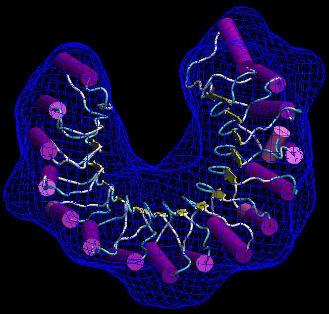
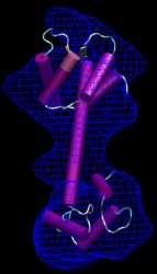
The result
should look like the following figure. Note the smooth surface that
wraps around the beadmodel without penetrating into it:
(Click
image to
enlarge)
(You can change the rendering style and transparency of the wrapped isocontour and PDB in the VMD Graphics menu).
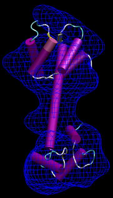
Now inspect the
alternative solution col_best_002.pdb. The second ribonuclease
inhibitor
structure is "flipped" about the pseudo-symmetry axis of the U-shaped
molecule.
This kind of degeneracy of the best fit can be expected in the case of
symmetric shapes. One
should expect unique fits only in cases where the shape of the molecule
clearly determines the registration.
As an additional exercise
you
may do the same
for troponin C using a 4Å bead radius.
|
Manual
Docking and
Refinement
In many fitting applications
an expert
user may have a pretty good idea where to place a biomolecule.
Therefore, manu users wish to manually dock atomic structures
into low resolution maps. (In VMD
one can move a
loaded molecule by selecting the menu Mouse -> Move ->
Molecule,
then translate it with the mouse and rotate it by pressing the Shift
key; the new coordinates can then be saved by selecting File ->
Save
Coordinates).
We
support this
manual docking by providing a refinement tool, collage, that performs a single optimization run to the nearest maximum of the
cross-correlation coefficient (if a refinement after manual docking is
desired). As with colores above, care
must be taken in the case of SAXS to always select standard correlation (option
"-corr 0"), since a possible default option (Laplacian
filter)
would
amplify the segmentation of the data caused by the SAXS beads. collage can take one or more PDB files as input.
Inspection of the troponin C
files
0_tnc.pdb and 1_tnc_sph.situs
reveals that 0_tnc.pdb
is
slightly misplaced relative to the volumetric map, although the
structures do overlap. This is a good start situation for manual
refinement with collage. Here we give the results of
a collage
run based on these two input files (note the -corr 0 and the resolution
-res 6.333 which is the value returned by the earlier pdb2vol
conversion of 1_tnc_sph.situs):
./collage
1_tnc_sph.situs 0_tnc.pdb -res 6.333 -corr 0
_____________________________________________________________________________
collage> Options read:
collage> Target resolution 6.333
collage> Resolution anisotropy 1.000
collage> Powell correlation algorithm determined automatically
collage> Low-resolution map cutoff 0.000
collage> Powell maximization ON
collage> Standard cross correlation
collage> Powell tolerance 1.00E-06 Max iterations 50
collage> Powell trans & rot initial step sizes set to default values
_____________________________________________________________________________
collage> Processing low-resolution map.
lib_vio> Situs formatted map file 1_tnc_sph.situs - Header information:
lib_vio> Columns, rows, and sections: x=1-90, y=1-46, z=1-45
lib_vio> 3D coordinates of first voxel: (-48.000000,-19.000000,-39.000000)
lib_vio> Voxel size in Angstrom: 1.000000
lib_vio> Reading density data...
lib_vio> Volumetric data read from file 1_tnc_sph.situs
lib_vwk> Map interpolated from 90 x 46 x 45 to 56 x 29 x 28.
lib_vwk> Voxel spacings interpolated from (1.000,1.000,1.000) to (1.583,1.583,1.583).
lib_vwk> New map origin (coord of first voxel), in register with coordinate system origin: (-47.498,-18.999,-37.998)
lib_vwk> Setting density values below 0.000000 to zero.
lib_vwk> Remaining occupied volume: 45472 voxels.
lib_vwk> Map size changed from 56 x 29 x 28 to 55 x 27 x 25.
lib_vwk> New map origin (coord of first voxel): (-47.498,-17.416,-36.415)
lib_vwk> Map density info: max 1.016194, min 0.000000, ave 0.133514, sig 0.273129.
_____________________________________________________________________________
collage> Processing atomic structures.
lib_pio> 1271 atoms read.
collage> One atomic input structure detected:
collage> 1. 0_tnc.pdb (1271 atoms)
_____________________________________________________________________________
lib_vwk> Generating Gaussian kernel with 7^3 = 343 voxels.
lib_vwk> Generating Gaussian kernel with 11^3 = 1331 voxels.
lib_vwk> Generating kernel with 7^3 = 343 voxels.
lib_vwk> Map size expanded from 55 x 27 x 25 to 61 x 33 x 31 by zero-padding.
lib_vwk> New map origin (coord of first voxel): (-52.247,-22.166,-41.165)
collage> Projecting probe structure to lattice...
collage> (no steric exclusion boosting of density)
collage> Computing fraction of PDB contained within the map (above cutoff density) ...
collage> Overlap fraction: 1.4844269E-01
collage> Warning: Less than half of the input PDB is contained within the map!
collage> Applying filters to target and probe maps...
collage> Normalizing target and probe maps...
collage> Target and probe maps:
lib_vwk> Map density info: max 4.056848, min 0.000000, ave 0.317103, sig 0.902745.
lib_vwk> Map density info: max 7.805456, min 0.000000, ave 0.257985, sig 0.937638.
collage> Initial correlation coefficient: 1.4506603E-01
_____________________________________________________________________________
collage> Identifying inside or buried voxels...
collage> Found 7696 inside or buried voxels (out of a total of 62403).
collage> Powell conjugent gradient maximization.
collage> Determining most efficient correlation algorithm based on convergence and time...
collage> Original algorithm: Correlation = 0.15601827 Time = 1.894500 ms
collage> Masked algorithm: Correlation = 0.12867513 Time = 1.853000 ms
collage> One-step algorithm: Correlation = 0.15139914 Time = 1.120000 ms
collage> Using original three-step correlation function.
collage>
collage> Performing Powell conjugate gradient maximization...
collage>
collage> Single-body Powell
collage> X
Y
Z Psi
Theta Phi
Correlation Iteration PDB (Body) Nr.
collage> 0.000 0.000
0.000 0.000 0.000
0.000 1.4506603E-01 Initial
1
collage> 2.284 -1.190 -18.364 36.872
11.519 328.383 6.3113920E-01
Final
1
collage> Total number of Powell steps: 26
collage> Total optimization time: 28.654045 s
_____________________________________________________________________________
collage> Writing body number 1 to file cge_001.pdb.
collage> Writing Powell log to file cge_powell.log.
_____________________________________________________________________________
collage> All done!!!
|
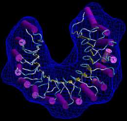
The
program output shows how
the
initial correlation of 0.1 increases to 0.6 while the structure is
fitted. The output is written to the file cge_best_001.pdb. To avoid
over writing this file, we create a directory "4_manual" and move the cge_* files into it (see run_tutorial.bash script).
When
inspected
with VMD as above, the results should look similar to the following
figure:
(Click
image to
enlarge)
|
| Outlook:
Alternative Fitting Strategies
Enforcing symmetry
The collage tool and the pdbsymm
tool can be combined to impose symmetry constraints on the
fragments during multi-fragment docking. Currently we
support C, D, and helical symmetry. This feature should be
very useful for many oligomeric assemblies. See the multi-fragment tutorial
for details.
Flexible
docking
It is well known
that proteins
can adopt a solution conformations that deviate from a known crystal
structure.
Consider e.g. the case of calmodulin which was first shown by SAXS to
compact
in solution (Heidorn & Trewhella, Biochemistry 1988 Feb 9;
27(3):
909-15)
and whose first solved crystal structure was not in the
"physiologically
relevant" conformation. For cases like this the flexible docking tools
described in the flexible
docking tutorial,
although developed with electron microscopy in mind, may also become
very useful to SAXS modelers.
|
| Return
to the front page . |
|