|
Multi-Fragment Docking Tutorial
|
| The tutorial shows the
manual
placement of structures into EM maps "by eye" and their subsequent
refinement with the collage
tool. The refinement examples shown include single fragment docking,
simultaneous multiple fragment docking, and multiple fragment docking
with symmetry enforced. The
results
can be compared to solutions distributed with the tutorial software.
More documentation is available in the user
guide, in the methodology
page, and in
the published articles. |
|
Content:
|
| Download
and Installation
First, follow these registration
and download steps (each Situs tutorial is separate and must
be downloaded and compiled individually)! Then, return to this page. The
Situs_3.1_multi_tutorial/bin directory will contain the executables as well as eight input data
files and an executable shell
script:
-
0_hexamer_reference.pdb:
For validating purposes, PDB entry 2REC.
- 0_hexamer.situs:
Simulated EM map
(Situs format) at 15Å resolution of the RecA hexamer (PDB
entry 2REC).
- 0_monomer_*.pdb: Atomic
(carbon alpha) coordinates
of slightly misplaced and rotated monomers (*=1-6) of RecA.
- run_tutorial.bash:
Bash shell script containing all commands of this tutorial (actually,
there is only one shell command here, the VMD scripts shown below are
more
important in this tutorial).
In
the
following, we will perform various modeling tasks.
The user can compare all generated files to the files in the
"solutions"
directory.
|
Data
Flow and Design
The
series
of steps and the utilities that are required for multi-fragment docking
are shown
schematically
in the following figure. Detailed program
explanations are
given
in the user guide.
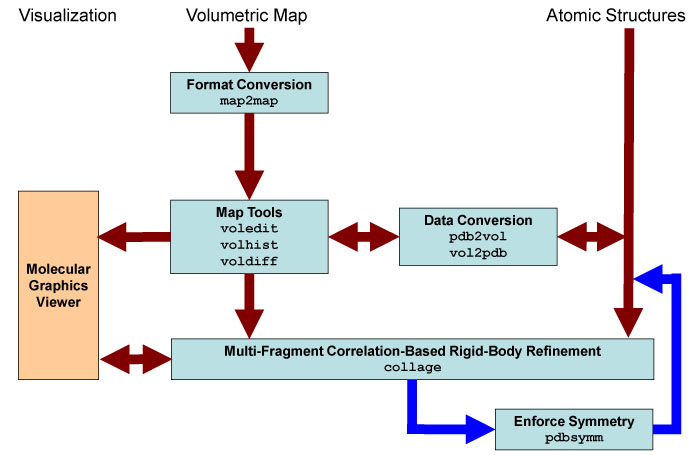
Schematic
diagram of collage-related
Situs components (light blue). The main data
flow is indicated by brown arrows. The optional enforcement of symmetry
with pdbsymm is
indicated by dark blue arrows. The visualization
(orange) requires an external molecular
graphics viewer (we use here the VMD
graphics program,
Chimera and Sculptor also
support Situs
format).
Standard
EM
formats are supported
and are converted to cubic lattices in Situs format. This is done with
the map2map
utility. Subsequently,
the data is inspected and, if necessary, prepared for the fitting using
a variety of visualization and analysis tools. The docking tool collage requires one
volume and one or more PDB structures for the fitting. Atomic
coordinates in PDB format can be transformed to low-resolution maps, if
necessary, and vice versa, to allow docking of maps to maps or
structures to structures. The
resulting docked complex can be inspected in the graphics program.
|
| Manual
Docking (Optional)
In many fitting applications
an expert
user may have a pretty good idea where to place a biomolecule.
Therefore, it is quite a popular approach to manually dock atomic
structures
into low resolution maps. In molecular graphics program such as VMD
one can shift and
rotate a
loaded molecule and save the new coordinates.
For convenience, the
following VMD
commands can be pasted directly into
the VMD command shell (cf. VMD
user
guide):
| vmd
shell
commands:
mol load
situs
0_hexamer.situs
mol load
pdb 0_monomer_1.pdb
mol load
pdb 0_monomer_2.pdb
mol load
pdb 0_monomer_3.pdb
mol load
pdb 0_monomer_4.pdb
mol load
pdb 0_monomer_5.pdb
mol load
pdb 0_monomer_6.pdb
mol top 0
rotate
stop
display
resetview
display
projection
orthographic
mol
modstyle 0 0
Isosurface 1 0 0 1 2 1
mol
modstyle 0 1
Trace 0.3 32
mol
modstyle 0 2
Trace 0.3 32
mol
modstyle 0 3
Trace 0.3 32
mol
modstyle 0 4
Trace 0.3 32
mol
modstyle 0 5
Trace 0.3 32
mol
modstyle 0 6
Trace 0.3 32
mol
modcolor 0 0
ColorID 0
mol
modcolor 0 1
ColorID 3
mol
modcolor 0 2
ColorID 3
mol
modcolor 0 3
ColorID 3
mol
modcolor 0 4
ColorID 3
mol
modcolor 0 5
ColorID 3
mol
modcolor 0 6
ColorID 3
|
 |
Don't forget to hit "enter"
after the last line! Exit VMD when done.
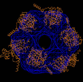
Notice how
the initial structures are misplaced relative to the map? We will
refine them shortly.
Then
select the VMD
menu
Mouse ->
Move -> Molecule. You can now click on individual monomer
structures with the
mouse
and rotate them by pressing the Shift
key; the new coordinates can then be saved to a file by selecting the
VMD menu File -> Save
Coordinates (select "all" atoms). Test this strategy and and create two
new PDB files as you wish (this optional exercise is not required for
the following refinement steps). |
Refinement
of Single Fragments
We support
manual docking by providing a tool, collage, that
calculates the
cross correlation (as a way to provide quantitative feedback) and
performs a single optimization run to the nearest maximum of the
cross-correlation coefficient (if a refinement after manual docking is
desired). As with colores, the
user
may select standard or Laplacian filtered correlation
explicitely (option
"-corr 0" or "-corr 1"), otherwise the default option
(resolution-dependent) is
applied.
The first monomer, 0_monomer_1.pdb, was
misplaced
and rotated relative to the volumetric map, but it is not too far from
the optimum. This is a good
start situation for manual
refinement with collage. Here we show the results of
a collage
run for the first monomer only (note the -corr 1 option, turning on the
Laplacian filter).
We also specify a resolution
15Å:
./collage
0_hexamer.situs 0_monomer_1.pdb -corr 1 -res 15
_____________________________________________________________________________
collage> Options read:
collage> Target resolution 15.000
collage> Resolution anisotropy 1.000
collage> Powell correlation algorithm determined automatically
collage> Low-resolution map cutoff 0.000
collage> Powell maximization ON
collage> Laplacian filtered correlation
collage> Powell tolerance 1.00E-06 Max iterations 50
collage> Powell trans & rot initial step sizes set to default values
_____________________________________________________________________________
collage> Processing low-resolution map.
lib_vio> Situs formatted map file 0_hexamer.situs - Header information:
lib_vio> Columns, rows, and sections: x=1-43, y=1-41, z=1-29
lib_vio> 3D coordinates of first voxel: (-84.000000,-80.000000,-68.000000)
lib_vio> Voxel size in Angstrom: 4.000000
lib_vio> Reading density data...
lib_vio> Volumetric data read from file 0_hexamer.situs
lib_vwk> Setting density values below 0.000000 to zero.
lib_vwk> Remaining occupied volume: 51127 voxels.
lib_vwk> Map size changed from 43 x 41 x 29 to 37 x 35 x 23.
lib_vwk> New map origin (coord of first voxel): (-72.000,-68.000,-56.000)
lib_vwk> Map density info: max 5.881478, min 0.000000, ave 0.709373, sig 1.280587.
_____________________________________________________________________________
collage> Processing atomic structures.
lib_pio> 303 atoms read.
collage> One atomic input structure detected:
collage> 1. 0_monomer_1.pdb (303 atoms)
_____________________________________________________________________________
lib_vwk> Generating Gaussian kernel with 7^3 = 343 voxels.
lib_vwk> Generating Gaussian kernel with 11^3 = 1331 voxels.
lib_vwk> Generating Laplacian kernel with 3^3 = 27 voxels.
lib_vwk> Generating kernel with 9^3 = 729 voxels.
lib_vwk> Map size expanded from 37 x 35 x 23 to 45 x 43 x 31 by zero-padding.
lib_vwk> New map origin (coord of first voxel): (-88.000,-84.000,-72.000)
collage> Projecting probe structure to lattice...
collage> (no steric exclusion boosting of density)
collage> Computing fraction of PDB contained within the map (above cutoff density) ...
collage> Overlap fraction: 9.8243647E-01
collage> Applying filters to target and probe maps...
lib_vwk> Relaxing 5 voxel thick shell about thresholded density...
collage> Normalizing target and probe maps...
collage> Target and probe maps:
lib_vwk> Map density info: max 6.002296, min -8.313631, ave -0.000097, sig 0.560120.
lib_vwk> Map density info: max 10.390867, min -18.678137, ave -0.006849, sig 0.475055.
collage> Initial correlation coefficient: -1.7409664E-02
_____________________________________________________________________________
collage> Identifying inside or buried voxels...
collage> Found 25657 inside or buried voxels (out of a total of 59985).
collage> Powell conjugent gradient maximization.
collage> Determining most efficient correlation algorithm based on convergence and time...
collage> Original algorithm: Correlation = -0.01132313 Time = 1.529500 ms
collage> Masked algorithm: Correlation = -0.01132313 Time = 1.425000 ms
collage> One-step algorithm: Correlation = -0.01145076 Time = 1.042500 ms
collage> Using masked three-step correlation function.
collage>
collage> Performing Powell conjugate gradient maximization...
collage>
collage> Single-body Powell
collage> X
Y
Z Psi
Theta Phi
Correlation Iteration PDB (Body) Nr.
collage> 0.000 0.000
0.000 0.000 0.000
0.000 -1.7409664E-02 Initial
1
collage> -2.154 -11.684 -1.559 40.020
4.057 313.739 3.9592493E-01
Final
1
collage> Total number of Powell steps: 11
collage> Total optimization time: 5.377984 s
_____________________________________________________________________________
collage> Writing body number 1 to file cge_001.pdb.
collage> Writing Powell log to file cge_powell.log.
_____________________________________________________________________________
collage> All done!!!
|
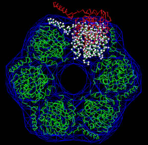
The
program output shows how the
initial correlation of -0.01 increases to 0.4 while the
structure is
matched (the correlation maximum is significantly below 1 due
to the fitting to much larger map and due to the use of the Laplacian).
The output is written to the file cge_001.pdb. We
rename
this file to "1_monomer_1.pdb" to avoid overwriting it later:
mv
cge_001.pdb 1_monomer_1.pdb
rm cge_*
|
To inspect the result (white
spheres) and to compare it to the initial conformation (red) and the
reference structure (green) the
following VMD
commands can be pasted directly into
the VMD command shell:
| vmd
shell
commands:
mol load
pdb
0_hexamer_reference.pdb
mol load
situs
0_hexamer.situs
mol load
pdb 1_monomer_1.pdb
mol load
pdb 0_monomer_1.pdb
mol top 0
rotate
stop
display
resetview
display
projection
orthographic
mol
modstyle 0 0
Trace 0.3 32
mol
modstyle 0 1
Isosurface 1 0 0 1 2 1
mol
modstyle 0 2 VDW 0.6 13
mol
modstyle 0 3
Trace 0.3 32
mol
modcolor 0 0
ColorID 7
mol
modcolor 0 1
ColorID 0
mol
modcolor 0 2
ColorID 8
mol
modcolor 0 3
ColorID 1
|
 |
Don't forget to hit "enter"
after the last line! Exit VMD when done.
Note
that the
correlation is the only criterion employed by collage. In some cases,
e.g. low
resolution or significant buried surface, the correlation criterion is
ambiguous or breaks down when
docking one fragment at a time. In such cases collage may actually
worsen the fit of single fragments.
The user should experiment in such challenging cases with various
parameters of the program, and with turning the Laplacian filter on or
off (-corr option). However, an even better strategy is to fit all
fragments simultaneously as described in the next two sections.
|
Refinement
of Multiple Fragments
In this
example we refine all six input monomers
simultaneously using standard correlation (-corr 0). collage
automatically detects the number of input PDB files if they are entered
in sequence:
./collage
0_hexamer.situs 0_monomer_1.pdb 0_monomer_2.pdb \
0_monomer_3.pdb 0_monomer_4.pdb
0_monomer_5.pdb \
0_monomer_6.pdb -corr 0 -res 15
_____________________________________________________________________________
collage> Options read:
collage> Target resolution 15.000
collage> Resolution anisotropy 1.000
collage> Powell correlation algorithm determined automatically
collage> Low-resolution map cutoff 0.000
collage> Powell maximization ON
collage> Standard cross correlation
collage> Powell tolerance 1.00E-06 Max iterations 50
collage> Powell trans & rot initial step sizes set to default values
_____________________________________________________________________________
collage> Processing low-resolution map.
lib_vio> Situs formatted map file 0_hexamer.situs - Header information:
lib_vio> Columns, rows, and sections: x=1-43, y=1-41, z=1-29
lib_vio> 3D coordinates of first voxel: (-84.000000,-80.000000,-68.000000)
lib_vio> Voxel size in Angstrom: 4.000000
lib_vio> Reading density data...
lib_vio> Volumetric data read from file 0_hexamer.situs
lib_vwk> Setting density values below 0.000000 to zero.
lib_vwk> Remaining occupied volume: 51127 voxels.
lib_vwk> Map size changed from 43 x 41 x 29 to 37 x 35 x 23.
lib_vwk> New map origin (coord of first voxel): (-72.000,-68.000,-56.000)
lib_vwk> Map density info: max 5.881478, min 0.000000, ave 0.709373, sig 1.280587.
_____________________________________________________________________________
collage> Processing atomic structures.
lib_pio> 303 atoms read.
lib_pio> 303 atoms read.
lib_pio> 303 atoms read.
lib_pio> 303 atoms read.
lib_pio> 303 atoms read.
lib_pio> 303 atoms read.
collage> Atomic input structures detected:
collage> 1. 0_monomer_1.pdb (303 atoms)
collage> 2. 0_monomer_2.pdb (303 atoms)
collage> 3. 0_monomer_3.pdb (303 atoms)
collage> 4. 0_monomer_4.pdb (303 atoms)
collage> 5. 0_monomer_5.pdb (303 atoms)
collage> 6. 0_monomer_6.pdb (303 atoms)
_____________________________________________________________________________
lib_vwk> Generating Gaussian kernel with 7^3 = 343 voxels.
lib_vwk> Generating Gaussian kernel with 11^3 = 1331 voxels.
lib_vwk> Generating kernel with 7^3 = 343 voxels.
lib_vwk> Map size expanded from 37 x 35 x 23 to 43 x 41 x 29 by zero-padding.
lib_vwk> New map origin (coord of first voxel): (-84.000,-80.000,-68.000)
collage> Projecting probe structure to lattice...
collage> (no steric exclusion boosting of density)
collage> Computing fraction of PDB contained within the map (above cutoff density) ...
collage> Overlap fraction: 9.2835467E-01
collage> Applying filters to target and probe maps...
collage> Normalizing target and probe maps...
collage> Target and probe maps:
lib_vwk> Map density info: max 4.991302, min 0.000000, ave 0.350711, sig 0.889630.
lib_vwk> Map density info: max 5.076604, min 0.000000, ave 0.366342, sig 0.885298.
collage> Initial correlation coefficient: 6.2730276E-01
_____________________________________________________________________________
collage> Identifying inside or buried voxels...
collage> Found 12101 inside or buried voxels (out of a total of 51127).
collage> Powell conjugent gradient maximization.
collage> Determining most efficient correlation algorithm based on convergence and time...
collage> Original algorithm: Correlation = 0.60949964 Time = 3.371500 ms
collage> Masked algorithm: Correlation = 0.60843375 Time = 3.875000 ms
collage> Using original three-step correlation function.
collage>
collage> Performing Powell conjugate gradient maximization...
collage>
collage> Multi-body Powell
collage> X
Y
Z Psi
Theta Phi
Correlation Iteration PDB (Body) Nr.
collage> 0.000 0.000
0.000 0.000 0.000
0.000 6.2730276E-01 Initial
1
collage> 0.000 0.000
0.000 0.000 0.000
0.000 6.2730276E-01 Initial
2
collage> 0.000 0.000
0.000 0.000 0.000
0.000 6.2730276E-01 Initial
3
collage> 0.000 0.000
0.000 0.000 0.000
0.000 6.2730276E-01 Initial
4
collage> 0.000 0.000
0.000 0.000 0.000
0.000 6.2730276E-01 Initial
5
collage> 0.000 0.000
0.000 0.000 0.000
0.000 6.2730276E-01 Initial
6
collage> -2.133 -11.769 -1.515 64.570
3.499 289.717 9.9922472E-01
Final
1
collage> 1.884 -6.191 -2.143
271.550 6.595 68.002 9.9922472E-01
Final
2
collage> -11.933 8.718 9.683
45.883 45.831 319.195 9.9922472E-01
Final
3
collage> 9.405 -7.100 -0.824
0.533 0.170 0.305
9.9922472E-01 Final
4
collage> 17.633 7.091 -3.219 217.267
39.768 140.325 9.9922472E-01
Final
5
collage> -10.788 -1.853 -2.001 174.526 19.379
192.758 9.9922472E-01
Final
6
collage> Total number of Powell steps: 30
collage> Total optimization time: 0 h 2 m 55 s
_____________________________________________________________________________
collage> Writing body number 1 to file cge_001.pdb.
collage> Writing body number 2 to file cge_002.pdb.
collage> Writing body number 3 to file cge_003.pdb.
collage> Writing body number 4 to file cge_004.pdb.
collage> Writing body number 5 to file cge_005.pdb.
collage> Writing body number 6 to file cge_006.pdb.
collage> Writing Powell log to file cge_powell.log.
_____________________________________________________________________________
collage> All done!!!
|
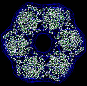
The
program output shows how the
initial correlation of 0.63 increases to 1 while the
structures are
matched.
The output structures are written to the files cge_*.pdb. We
rename
these files to "2_monomer_*.pdb" to avoid overwriting them later:
mv
cge_001.pdb 2_monomer_1.pdb
mv cge_002.pdb 2_monomer_2.pdb
mv cge_003.pdb 2_monomer_3.pdb
mv cge_004.pdb 2_monomer_4.pdb
mv cge_005.pdb 2_monomer_5.pdb
mv cge_006.pdb 2_monomer_6.pdb
rm cge_*
|
To inspect the results
(white
spheres) and to compare them to the
reference structure (green) the
following VMD
commands can be pasted directly into
the VMD command shell:
| vmd
shell
commands:
mol load
pdb
0_hexamer_reference.pdb
mol load
situs
0_hexamer.situs
mol load
pdb 2_monomer_1.pdb
mol load
pdb 2_monomer_2.pdb
mol load
pdb 2_monomer_3.pdb
mol load
pdb 2_monomer_4.pdb
mol load
pdb 2_monomer_5.pdb
mol load
pdb 2_monomer_6.pdb
mol top 0
rotate
stop
display
resetview
display
projection
orthographic
mol
modstyle 0 0
Trace 0.3 32
mol
modstyle 0 1
Isosurface 1 0 0 1 2 1
mol
modstyle 0 2 VDW 0.6 13
mol
modstyle 0 3 VDW 0.6 13
mol
modstyle 0 4 VDW 0.6 13
mol
modstyle 0 5 VDW 0.6 13
mol
modstyle 0 6 VDW 0.6 13
mol
modstyle 0 7 VDW 0.6 13
mol
modcolor 0 0
ColorID 7
mol
modcolor 0 1
ColorID 0
mol
modcolor 0 2
ColorID 8
mol
modcolor 0 3
ColorID 8
mol
modcolor 0 4
ColorID 8
mol
modcolor 0 5
ColorID 8
mol
modcolor 0 6
ColorID 8
mol
modcolor 0 7
ColorID 8
|
 |
Don't forget to hit "enter"
after the last line! Exit VMD when done.
In
this example we did not enforce six-fold (C6) symmetry. This option
will be described in the
next section.
|
Refinement
of Multiple Fragments with Symmetry Enforced
Symmetry
constraints are outsourced to a separate program in the UNIX shell
script. You have two choices for enforcing symmetry with collage:
- You can use our pdbsymm
tool that allows to create multiple symmetry related copies of monomers.
Currently supported are C, D, and H (helical) symmetry.
- For
other specialized cases (various icosahedral conventions,
crystallographic, etc) it is likely that you already have a tool
for creating symmetry copies from a PDB which you may subsitute
for pdbsymm in the following.
Our
goal is to keep Situs tools modular, and to avoid having to write
specialized tools for every possible symmetry scenario. This means that
collage will technically still treat each fragment as independent. But we will take only a single conjugate gradient step, and after each step the symmetry will again be enforced. The net effect after several iterations is a symmetry-enforced conjugate gradient optimization.
Here is our work flow for the UNIX shell script implementation:
- Define
which input structure is the initial master monomer.
- Generate
symmetry copies from the master monomer with pdbsymm (or your own tool).
- Extract
individual symmetry copies from the output file using the UNIX grep command.
- Refine
symmetry copies with collage using only
a single conjugate gradient step. Save
master monomer.
- Repeat
(loop) steps 2.-4. a couple of times (check convergence).
- Generate
final symmetry copies from master monomer using pdbsymm (or your own tool).
Below you find a UNIX bash script that implements this strategy using pdbsymm. You can paste this example directly into a bash shell (or modify it for your own needs). There are 20 loop iterations in this
example, and collage has been
restricted to only 1 optimization step per iteration with the -pwti flag:
#
initialize, set master monomer
rm curr_mon.pdb
cp 0_monomer_1.pdb curr_mon.pdb
# loop a few times alternating between pdbsymm and collage
for i in {1..20}
do
./pdbsymm curr_mon.pdb 0_hexamer.situs tmp.pdb
<<< 'C
6'
cat tmp.pdb | grep " 0 1"
> tmp1.pdb
cat tmp.pdb | grep " 0 2"
> tmp2.pdb
cat tmp.pdb | grep " 0 3"
> tmp3.pdb
cat tmp.pdb | grep " 0 4"
> tmp4.pdb
cat tmp.pdb | grep " 0 5"
> tmp5.pdb
cat tmp.pdb | grep " 0 6"
> tmp6.pdb
./collage 0_hexamer.situs tmp1.pdb tmp2.pdb tmp3.pdb
tmp4.pdb \
tmp5.pdb tmp6.pdb -corr 0 -res 15 -pwti 1e-6 1
mv -f cge_001.pdb curr_mon.pdb
rm tmp*.pdb
rm cge_*
done
# clean up
./pdbsymm curr_mon.pdb 0_hexamer.situs 3_final_hexamer.pdb
<<< 'C
6'
rm curr_mon.pdb
|
You can
find this protocol in the run_tutorial.bash script.
For convenience, in pdbsymm the
symmetry axes can be defined by an (optional) input map. But care must
be taken that the symmetry axis is at the map center defined in the user guide (crop or pad the
map
with voledit if
necessary). Here,
the C6 symmetry axis is conveniently oriented in the z direction and it is
centered in the x-y plane of the input map 0_hexamer.situs.
Run
this example and check the single output file, 3_final_hexamer.pdb,
which now contains all symmetry copies.
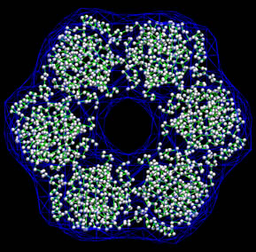
To inspect the result
(white
spheres) and to compare it to the
reference structure (green) the
following VMD
commands can be pasted directly into
the VMD command shell:
| vmd
shell
commands:
mol load
pdb
0_hexamer_reference.pdb
mol load
situs
0_hexamer.situs
mol load
pdb 3_final_hexamer.pdb
mol top 0
rotate
stop
display
resetview
display
projection
orthographic
mol
modstyle 0 0
Trace 0.3 32
mol
modstyle 0 1
Isosurface 1 0 0 1 2 1
mol
modstyle 0 2 VDW 0.6 13
mol
modcolor 0 0
ColorID 7
mol
modcolor 0 1
ColorID 0
mol
modcolor 0 2
ColorID 8
|
 |
As before, don't forget to
hit "enter"
after the last line!
|
| Return
to the front page. |
|