• Registration of Two Maps
• Density Histogram Matching of Two Registered Maps
• Map Averaging
• Unequal Size Point-Cloud Registration

As a prerequisite to density histogram matching, two maps must be brought into register to maximize the density cancellation zone (Wriggers et al, 2011). Here we use the output files 4_s1.situs and 4_s2.situs from part I as target and probe maps. Situs docking tools require an atomic structure (probe) and a density map (target), so the probe map must be first made movable by creating a pseudo-PDB file with vol2pdb. 

Finally, we map the rotated and translated probe back to the grid of the target map using pdb2vol. In the following session we select a voxel spacing of 6Å as before:

enter the number of histogram bins (30). Next, enter the surface value 20 for file 4_s1.situs and a value of 12 for file 6_s2.dock.situs (see part I of this tutorial). These surface isovalues will be automatically matched. Subsequently, the user has the uption of entering various bias values to interactively center the central peak of the difference histogram. We find that a bias value of -4.0 (corresponding to a gain factor of 2.0) provides for a well centered central peak. To save the transformation of 6_s2.dock.situs to the file tmp.situs, enter any value above 20.

We wish to use the map averaging tool volaver to build up a combined map from the (original, undocked) 4_s1.situs and 4_s2.situs monomer maps, where the "weaker" density of 4_s2.situs is subject to affine transformation with gain 2.0 and bias -4.0. This "strengthening" of the weaker monomer is necessary to give both of them equal weight in the docking below. To apply the affine transformation to 4_s2.situs, call volhist with only two arguments:

Note how the cutoff density in the histogram was moved from 12 to 20 (as in 4_s1.situs, which you can check with "./volhist 4_s1.situs" using only one argument).

Now we are finally ready to combine the monomer densities from both maps into a single "dimer" target map. The maps can be added using the volaver tool (subject to normalization by factor 2). At the prompt enter:

We now dock the high-resolution ncd structure into the larger dimer map with the matchpt utility. The dimer map fits exactly two input structures so we set the -units option to 2.0 (in general, this parameter may be non-integer). We also sort here the solutions by cross-correlation (CC) value using the "-ranking 1" option:

The best solutions in this list (by CC value) are mpt_001.pdb and mpt_002.pdb. These are nearly identical to the solutions found earlier (files 5_s2_1.dock.pdb and 5_s1_1.dock.pdb). 

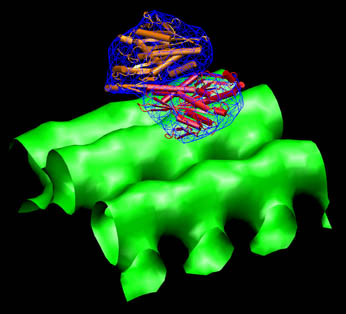
The following sequence of commands in the VMD text console (cf. VMD user guide) will load the two best solutions (red and orange), the microtubule surface (green), and the histogram matched dimer map (blue), and render them similarly to the final result in part I:

Don't forget to hit "enter" after the last line! 

The result should look like this:

Note: As described in (Birmanns & Wriggers, 2007), the fast point cloud matching can be improved by a post-processing with the fast correlation-based tool collage. We have explained this workflow in the separate multi-dock tutorial.