|
Tutorial
|
| This
tutorial shows how to use
FilaSitus programs with VMD to greate actin filaments
at
low resolution in a triangular bundle and side-by-side arrangement. The
created files can be compared with precomputed files provided in the
FilaSitus
solutions
directory.
More documentation is also available in the
User
Guide, the
Methodology
page of Situs, the VMD
user guide, and in the published
Situs articles. |
|
Content
|
| Creating
Atomic Structures of Actin Filament Bundles with filabuild
The filabuild
tool generates multiple copies of the input PDB file in the z-direction
according to a user-specified helical symmetry, and in the (x,y)
direction,
according to a specified offset. All helical parameters, the start
angle, flipping of filaments, etc., can be adjusted by the user in the
configuration
files.
Here we show how this is
done
with the provided input files. At the shell prompt, enter (you
can cut and paste this):
./filabuild
nohy_start_sd1.pdb configure_36_17_bundle.dat
13_sd1_bundle.pdb
./filabuild nohy_start_sd1.pdb configure_36_17_sidebyside.dat
13_sd1_sidebyside.pdb
./filabuild nohy_start.pdb configure_36_17_bundle.dat
13_bundle.pdb
./filabuild nohy_start.pdb configure_36_17_sidebyside.dat
13_sidebyside.pdb
|
The
first
two commands create filaments from actin's subdomain 1 (SD1) only,
whereas
the last two generate the full structures. To
learn the functionality of the program, you
can inpect the resulting
stuctures with VMD. You can explore the appearance of
the structures depending on the specified parameters that are
documented
in the configuration files.
We
have
now created structures of full actin and SD1, both as a triangular
bundle,
and side-by-side. Note that the angle (phase) offsets were adjusted
between bundle and side-by-side to reflect the correct orientation of
the
filaments when the triangular bundle is "folded" open to show the
interior
contacts.
|
| Creating
Low-Resolution Volumetric (Simulated EM) Data with kercon
To create a visually
appealing
low-resolution representation of the atomic structures, we use the kercon
tool to project them to a cubic lattice and to convolve the resulting
3D density
with a Gaussian blurring kernel at a user-specified resolution. Here,
we
take the 4 structures created above and blur them to a resolution of
20A,
although smaller values can be entered to reveal more spatial detail.
The
choice of resolution is up to the user.
Here we show how this is
done with one of the structures. At the shell prompt, enter:
| ./kercon
13_bundle.pdb 13_bundle.situs |
Next,
at
the program prompt, enter 2 (mass density blurring), the desired voxel
spacing of the lattice: 6 (A), the desired kernel: 1 (Gaussian), target
resolution: 20 (A), kernel amplitude: 1 (this is arbitrary, different
values
give a different scaling of the 3D density), sigma correction: 1. Here
is the complete output of this run:
./kercon 13_bundle.pdb 13_bundle.situs
pdbio> 124404 atoms read.
kercon> What kind of 3D density function do you want to create:
kercon>
kercon> 1: Charge density (atom charges will be read from PDB occupancy field)
kercon> 2: Mass density (atom masses are assigned automatically)
kercon> 2
kercon> There are 124404 non-hydrogen atoms, represented by 125370 equally weighted input atoms
kercon>
kercon> The input structure measures 174.508 x 163.790 x 420.297 Angstrom
kercon>
kercon> Please enter the desired voxel spacing for the output map (in Angstrom): 6
kercon>
kercon> Please select the type of kernel:
kercon>
kercon> 1: Gaussian: A exp(-1.5 r^2 / sigma^2),
kercon> useful for resolution-lowering of atomic structures.
kercon>
kercon> 2: Hard Sphere: 0 (outside) or A (inside),
kercon> useful for bead-modeling at reduced complexity:
kercon> - sphere radii are read from input PDB file (B-factor field).
kercon> - sphere boundaries are anti-aliased 1-voxel wide
kercon> 1
kercon> Kernel width. Please enter (in Angstrom):
kercon> (as pos. value) target resolution (== 2 sigma) or
kercon> (as neg. value) kernel half-max radius
kercon> Now enter (signed) value: 20
kercon>
kercon> The Gaussian kernel has the following properties:
kercon>
kercon> Gaussian, A exp(-1.5 r^2 / sigma^2)
kercon> sigma = 10.000A, r-half = 6.798A, r-cut = 17.321A
kercon>
kercon> Please enter the desired kernel amplitude A: 1
kercon>
kercon> Do you want to correct sigma for spreading introduced by tri-linear projection to lattice?
kercon>
kercon> 1: Yes (slightly lowers the kernel width to maintain target resolution)
kercon> 2: No
kercon> 1
kercon> Projecting atom masses to cubic lattice by tri-linear interpolation...
kercon> ... done. Lattice spread (rmsd): 4.244 Angstrom
kercon>
kercon> Computing Gaussian kernel (correcting sigma for lattice smoothing)...
kercon> ... done. Kernel map extent 7 x 7 x 7 voxels
kercon>
kercon> Convolving lattice with kernel...
kercon> ... done. Spatial resolution (2 sigma) of output map: 20.000A
kercon>
volio> Writing density data...
volio> Volumetric data written to file 13_bundle.situs
volio> File 13_bundle.situs - Header information:
volio> Columns, rows, and sections: x=1-41, y=1-39, z=1-82
volio> 3D coordinates of first voxel (1,1,1): (-78.000000,-78.000000,-66.000000)
volio> Voxel size in Angstrom: 6.000000
|
Again,
the
user can change some of the program parameters if desired. In the case
at hand one would probably only be interested in the effect of changing
resolution. As an exercise, repeat the same procedure for the input
structures
13_sidebyside.pdb,
13_sd1_bundle.pdb,
and 13_sd1_sidebyside.pdb, creating the
corresponding output maps
in Situs format: 13_sidebyside.situs,
13_sd1_bundle.situs,
and 13_sd1_sidebyside.situs, respectively.
|
| Visualizing
Isocontours with VMD
Now
we can load the isocontour
surfaces into VMD. For convenience, the following VMD commands can be
pasted
directly into the VMD command console:
mol
load situs 13_bundle.situs
mol
load situs 13_sd1_bundle.situs
mol modstyle 0 0 Isosurface 40 0 0 0 1 1
mol
modstyle 0 1 Isosurface 35 0 0 0 1 1
mol modcolor 0 0 ColorID 0
mol
modcolor 0 1 ColorID 1
display
resetview |
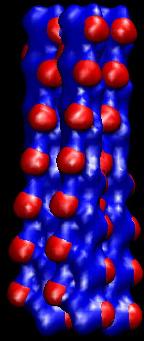
Here
is the view created by this
representation (note that you van make snapshots with the VMD File->Render
menu):
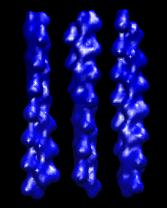
Similarly,
we can visualize the
side-by-side representation (open a new VMD session):
mol
load situs 13_sidebyside.situs
mol
load situs 13_sd1_sidebyside.situs
mol modstyle 0 0 Isosurface 40 0 0 0 1 1
mol
modstyle 0 1 Isosurface 35 0 0 0 1 1
mol modcolor 0 0 ColorID 0
mol
modcolor 0 1 ColorID 1
display
resetview
|
Here
is the view created by this
representation:
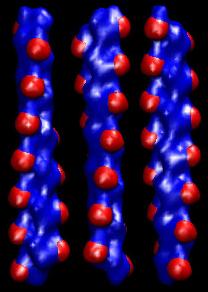
We
chose an isovalue of 40 because the
resulting blue surfaces appear similar to the molecular
surface of the actin filaments (see below). Also, we chose a slightly
smaller isolevel 35 for the red SD1
surfaces so that they occlude the surfaces of the full actin
filaments.
|
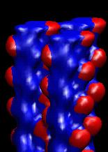
| Cropping
Maps with pindown
The surfaces created in the
above
manner are somewhat uneven at the ends of the filament, due to the
effect
of the blurring on the finite-size structures. One may wish to crop the
density files to trim off the filament ends to create a cleaner look.
This
has to be done on the Situs formatted files, i.e. before the
isocontours
are created. The suitable map cropping tool is pindown,
which allows one to extract a box of interest based on an enumeration
of
the lattice points. We enter one caveat here: Since the Situs formatted
maps may differ in their size and origin (3D coordinates of the [1,1,1]
voxel), one has to calculate at which lattice index to crop to create
similar appearance in two related files (e.g. in full actin and SD1).
To facilitate this calculation, the pindown program displays the map
parameters such as voxel spacing, origin and the number
of x, y, and z increments.
For a clean cropping of
the
ends on the data at hand we suggest the following: At the UNIX shell
prompt
enter e.g. (similar for the other files):
| ./pindown 13_bundle.situs
13_bundle_crop.situs |
At
the pindown prompt enter
the following crop regions: 1-41,1-39,15-67 (13_bundle_crop.situs),
1-41,1-39,13-65 (13_sd1_bundle_crop.situs),
1-61,1-27,15-67
(13_sidebyside_crop.situs), and 1-61,1-27,13-65 (13_sd1_sidebyside_crop.situs).
One can then visualize
the cropped density data (detail view):
For more general map editing
purposes we recommend the newer tools (such as voledit, volhist,
voldiff, etc) distributed with Situs.
|
| Creative
Use of the VMD Clipping Plane
The side-by-side
representation
is useful as it allows one to clip away any unwanted parts of the
molecular
surfaces with the VMD clipping plane. To test this, load again 13_sidebyside.situs
and 13_sd1_sidebyside.situs
as above. Now use the VMD "Far Clip" plane (VMD
Display
Menu / Display Settings) and bring it closer to the front. Take a
snapshot with the VMD Render tool. Next toggle off 3_sd1_sidebyside.situs
and
set the clipping plane behind the scene. Take a second snapshot. In
image editing programs like Adobe Photoshop you can make the black
background
of the first snapshot transparent and superimpose the colored pixels as
a layer onto the second snapshot. This should look as follows:
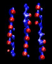 + +
 = = 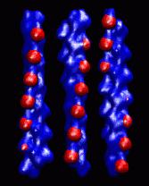
This is
a quick way to viualize the SD1 contacts in the center of the
triangular
bundle, if the phase offset angles of the side-by-side representation
were
chosen accordingly.
|
| Return
to the front page. |
|